ggNetView is an R package for network analysis and visualization. It provides flexible and publication-ready tools for exploring complex biological and ecological networks.
Installation
You can install the development version of ggNetView from GitHub with:
Example1
Step1: load ggNetView
library(ggplot2)
#> Warning: package 'ggplot2' was built under R version 4.5.2
library(ggnewscale)
library(ggNetView)
#>
#>                                                ░██               ░██
#>                                                ░██
#>  ░████████  ░████████ ░████████   ░███████  ░████████ ░██    ░██ ░██ ░███████  ░██    ░██    ░██
#> ░██    ░██ ░██    ░██ ░██    ░██ ░██    ░██    ░██    ░██    ░██ ░██░██    ░██ ░██    ░██    ░██
#> ░██    ░██ ░██    ░██ ░██    ░██ ░█████████    ░██     ░██  ░██  ░██░█████████  ░██  ░████  ░██
#> ░██   ░███ ░██   ░███ ░██    ░██ ░██           ░██      ░██░██   ░██░██          ░██░██ ░██░██
#>  ░█████░██  ░█████░██ ░██    ░██  ░███████      ░████    ░███    ░██ ░███████     ░███   ░███
#>        ░██        ░██
#>  ░███████   ░███████
#>
#>
#> Yue Liu, Chao Wang (2026). ggNetView: An R Package for Reproducible and Deterministic Network Analysis and Visualization.
#>
#>   Maintainers:
#>    - Yue Liu <yueliu@iae.ac.cn>
#>    - Chao Wang <cwang@iae.ac.cn>
#>
#>   Manual: https://jiawang1209.github.io/ggNetView-manual/
#>   GitHub: https://github.com/Jiawang1209/ggNetView
#>   Bug Reports: https://github.com/Jiawang1209/ggNetView/issues
#>
#>
#>   Type citation('ggNetView') for how to cite this package.
#>   Run browseVignettes('ggNetView') for documentation.
#>
Step2: load Data
You can load raw matrix
data("otu_tab")

otu_tab[1:5, 1:5]
#>        KO1  KO2  KO3  KO4  KO5
#> ASV_1 1113 1968  816 1372 1062
#> ASV_2 1922 1227 2355 2218 2885
#> ASV_3  568  460  899  902 1226
#> ASV_4 1433  400  535  759 1287
#> ASV_6  882  673  819  888 1475
You can load rarely matrix. Note : the rownames of
otu_rareis the features.
data("otu_rare")

otu_tab[1:5, 1:5]
#>        KO1  KO2  KO3  KO4  KO5
#> ASV_1 1113 1968  816 1372 1062
#> ASV_2 1922 1227 2355 2218 2885
#> ASV_3  568  460  899  902 1226
#> ASV_4 1433  400  535  759 1287
#> ASV_6  882  673  819  888 1475
data("otu_rare_relative")

otu_rare_relative[1:5, 1:5]
#>              KO1        KO2        KO3        KO4        KO5
#> ASV_1 0.03306667 0.05453333 0.02013333 0.03613333 0.02686667
#> ASV_2 0.05750000 0.03393333 0.06046667 0.05810000 0.07320000
#> ASV_3 0.01733333 0.01296667 0.02290000 0.02336667 0.03106667
#> ASV_4 0.04266667 0.01093333 0.01416667 0.01933333 0.03346667
#> ASV_6 0.02646667 0.01856667 0.02110000 0.02353333 0.03806667
You can load node annotation. Note : the rownames of
tax_tabis NULL.
data("tax_tab")

tax_tab[1:5, 1:5]
#> # A tibble: 5 × 5
#>   OTUID  Kingdom  Phylum          Class          Order
#>   <chr>  <chr>    <chr>           <chr>          <chr>
#> 1 ASV_2  Archaea  Thaumarchaeota  Unassigned     Nitrososphaerales
#> 2 ASV_3  Bacteria Verrucomicrobia Spartobacteria Unassigned
#> 3 ASV_31 Bacteria Actinobacteria  Actinobacteria Actinomycetales
#> 4 ASV_27 Archaea  Thaumarchaeota  Unassigned     Nitrososphaerales
#> 5 ASV_9  Bacteria Unassigned      Unassigned     Unassigned
Step3: create graph object
obj <- build_graph_from_mat(
  mat = otu_rare_relative,
  transfrom.method = "none",
  method = "WGCNA",
  cor.method = "pearson",
  proc = "BH",
  r.threshold = 0.7,
  p.threshold = 0.05,
  node_annotation = tax_tab
)

obj
#> # A tbl_graph: 2049 nodes and 9602 edges
#> #
#> # An undirected simple graph with 100 components
#> #
#> # Node Data: 2,049 × 14 (active)
#>    name    modularity modularity2 modularity3 Modularity Degree Strength Kingdom
#>    <chr>   <fct>      <ord>       <chr>       <ord>       <dbl>    <dbl> <chr>
#>  1 ASV_916 1          1           1           1              58     50.5 Bacter…
#>  2 ASV_777 1          1           1           1              58     48.7 Bacter…
#>  3 ASV_606 1          1           1           1              55     45.8 Bacter…
#>  4 ASV_740 1          1           1           1              54     47.2 Bacter…
#>  5 ASV_14… 1          1           1           1              54     44.5 Bacter…
#>  6 ASV_23… 1          1           1           1              54     47.4 Bacter…
#>  7 ASV_15… 1          1           1           1              52     45.3 Bacter…
#>  8 ASV_24… 1          1           1           1              52     43.0 Bacter…
#>  9 ASV_19… 1          1           1           1              52     43.0 Bacter…
#> 10 ASV_568 1          1           1           1              51     45.1 Bacter…
#> # ℹ 2,039 more rows
#> # ℹ 6 more variables: Phylum <chr>, Class <chr>, Order <chr>, Family <chr>,
#> #   Genus <chr>, Species <chr>
#> #
#> # Edge Data: 9,602 × 5
#>    from    to weight correlation corr_direction
#>   <int> <int>  <dbl>       <dbl> <chr>
#> 1  1771  1825  0.793       0.793 Positive
#> 2   594   597  0.895       0.895 Positive
#> 3   588   597  0.864       0.864 Positive
#> # ℹ 9,599 more rows
Step4: ggNetView to plot
Basic network plot
p1 <- ggNetView(
  graph_obj = obj,
  layout = "gephi",
  layout.module = "adjacent",
  group.by = "Modularity",
  fill.by = "Modularity",
  pointsize = c(1, 5),
  center = F,
  jitter = F,
  mapping_line = F,
  shrink = 0.9,
  linealpha = 0.2,
  linecolor = "#d9d9d9"
)

p1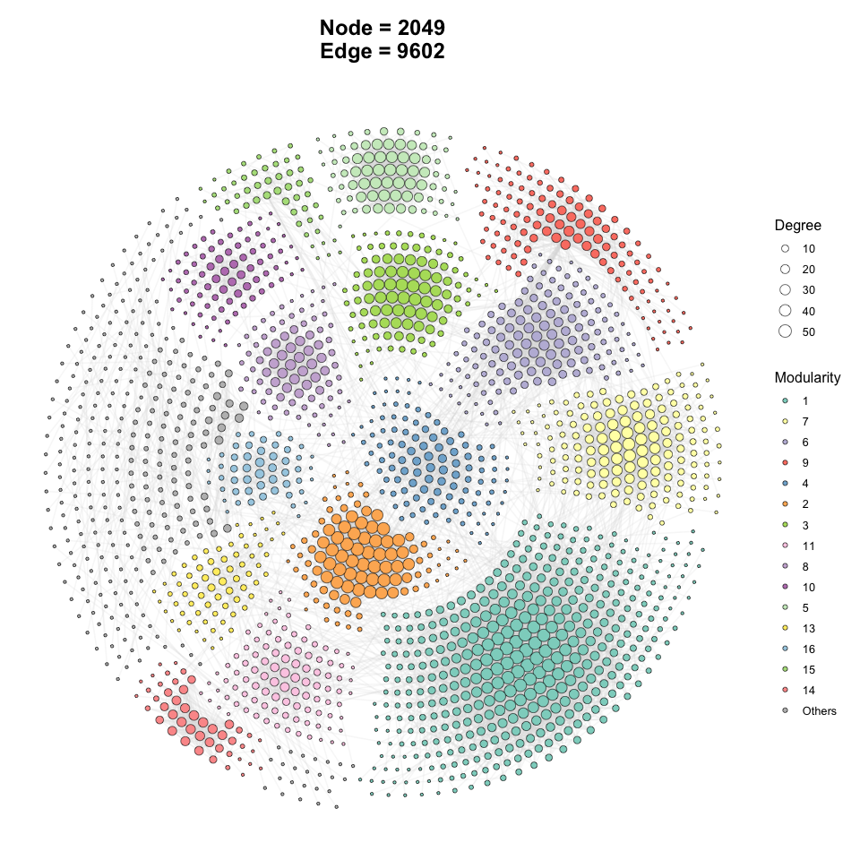
Add outer line in netwotk plot
p2 <- ggNetView(
  graph_obj = obj,
  layout = "gephi",
  layout.module = "adjacent",
  group.by = "Modularity",
  fill.by = "Modularity",
  pointsize = c(1, 5),
  center = F,
  jitter = TRUE,
  jitter_sd = 0.15,
  mapping_line = TRUE,
  shrink = 0.9,
  linealpha = 0.2,
  linecolor = "#d9d9d9",
  add_outer = T,
  label = T
)
#> Coordinate system already present.
#> ℹ Adding new coordinate system, which will replace the existing one.

p2
#> Warning: No shared levels found between `names(values)` of the manual scale and the
#> data's fill values.
Change the fill of node points.
p3 <- ggNetView(
  graph_obj = obj,
  layout = "gephi",
  layout.module = "adjacent",
  group.by = "Modularity",
  fill.by = "Phylum",
  pointsize = c(1, 5),
  center = F,
  jitter = TRUE,
  jitter_sd = 0.15,
  mapping_line = TRUE,
  shrink = 0.9,
  linealpha = 0.2,
  linecolor = "#d9d9d9",
  add_outer = T,
  label = T
)
#> Coordinate system already present.
#> ℹ Adding new coordinate system, which will replace the existing one.

p3
#> Warning: No shared levels found between `names(values)` of the manual scale and the
#> data's fill values.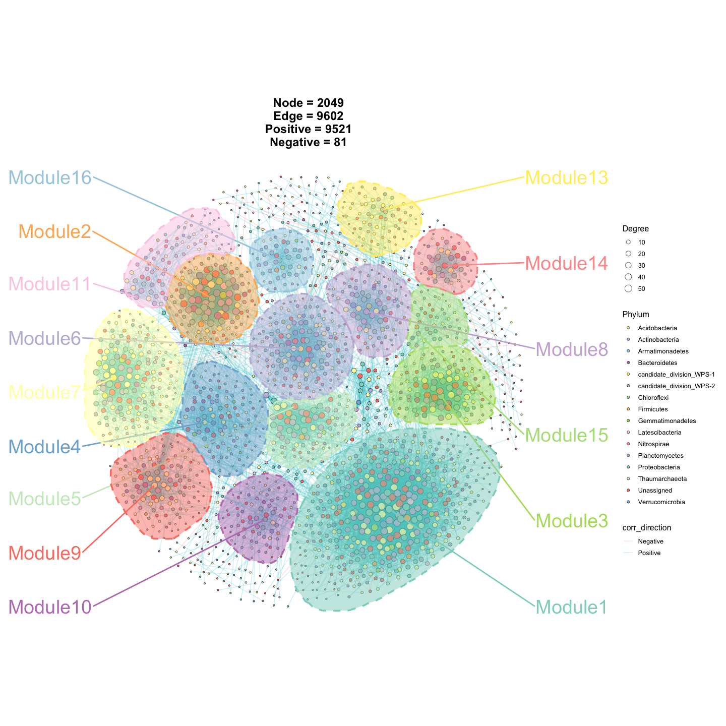
Change the color of node points.
p4 <- ggNetView(
  graph_obj = obj,
  layout = "gephi",
  layout.module = "adjacent",
  group.by = "Modularity",
  fill.by = "Phylum",
  color.by = "Phylum",
  pointsize = c(1, 5),
  center = F,
  jitter = TRUE,
  jitter_sd = 0.15,
  mapping_line = TRUE,
  shrink = 0.9,
  linealpha = 0.2,
  linecolor = "#d9d9d9",
  add_outer = T,
  label = T
)
#> Coordinate system already present.
#> ℹ Adding new coordinate system, which will replace the existing one.

p4
#> Warning: No shared levels found between `names(values)` of the manual scale and the
#> data's fill values.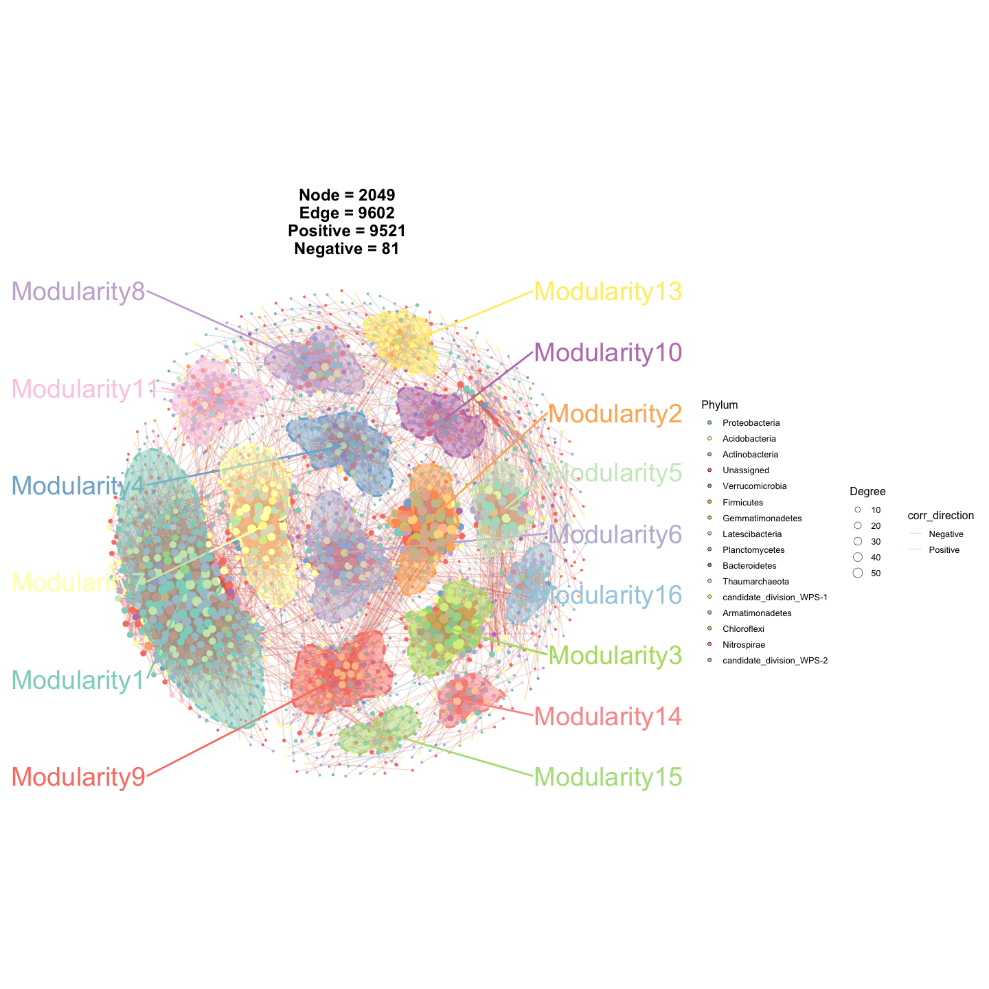
Add node label
p5 <- ggNetView(
  graph_obj = obj,
  layout = "gephi",
  layout.module = "adjacent",
  group.by = "Modularity",
  fill.by = "Modularity",
  pointsize = c(1, 5),
  center = F,
  jitter = TRUE,
  jitter_sd = 0.15,
  mapping_line = TRUE,
  shrink = 0.9,
  linealpha = 0.2,
  linecolor = "#d9d9d9",
  add_outer = T,
  label = T,
  pointlabel = "top1"
)
#> Coordinate system already present.
#> ℹ Adding new coordinate system, which will replace the existing one.

p5
#> Warning: No shared levels found between `names(values)` of the manual scale and the
#> data's fill values.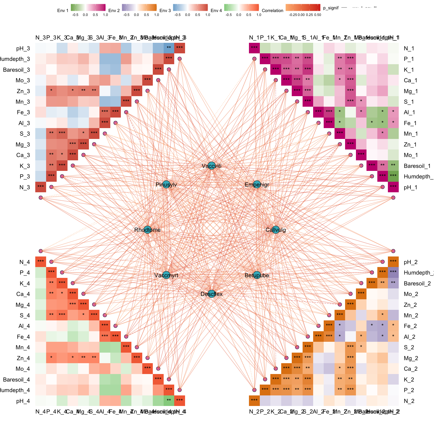
Example2
Get information of graph_object
Sub_module_1 <- get_subgraph(graph_obj = obj, select_module = "1")
#>    Module Number
#> 1       1    416
#> 2       7    161
#> 3       6    137
#> 4       9    121
#> 5       4    112
#> 6       2    105
#> 7       3    104
#> 8      11    101
#> 9       8     87
#> 10     10     80
#> 11      5     78
#> 12     13     70
#> 13     16     52
#> 14     15     51
#> 15     14     46
#> 16 Others    328

names(Sub_module_1)
#> [1] "sub_graph_all"    "stat_module"      "sub_graph_select"
Example3
out1 <- gglink_heatmaps(
  env = Envdf_4st,
  spec = Spedf,
  env_select = list(Env01 = 1:14,
                    Env02 = 15:28,
                    Env03 = 29:42,
                    Env04 = 43:56),
  spec_select = list(Spec01 = 1:8),
  relation_method = "correlation",
  spec_layout = "circle_outline",
  cor.method = "pearson",
  cor.use = "pairwise",
  r = 6,
  distance = 1,
  orientation = c("top_right", "bottom_right", "top_left", "bottom_left")
)
#> The max module in network is 2 we use the 2  modules for next analysis

out1[[1]]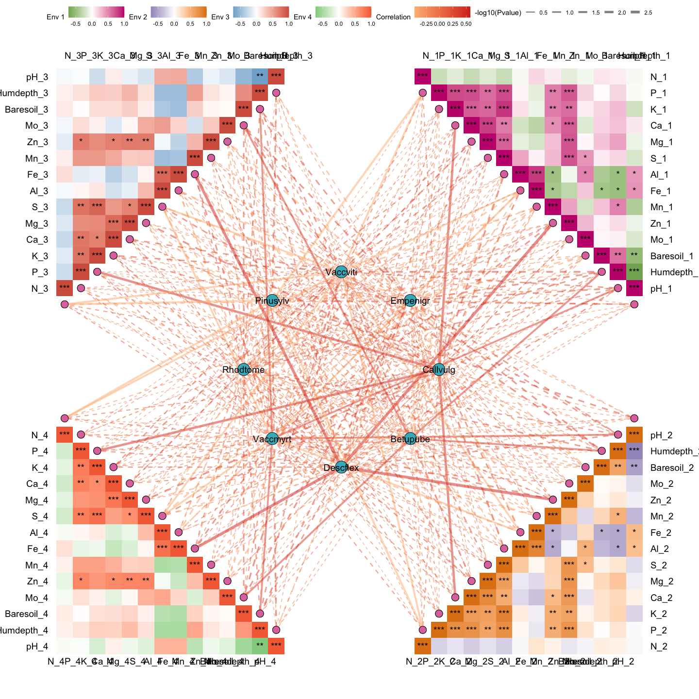
Example4
Leave lines with a significance level less than 0.05, and change the color of heatmap.
out2 <- gglink_heatmaps(
  env = Envdf_4st,
  spec = Spedf,
  env_select = list(Env01 = 1:14,
                    Env03 = 29:40,
                    Env04 = 43:50),
  spec_select = list(Spec01 = 1:8),
  relation_method = "correlation",
  spec_layout = "circle_outline",
  cor.method = "pearson",
  cor.use = "pairwise",
  drop_nonsig = TRUE,
  HeatmapColorBar = list(c("#2166ac", "#b2182b"),
                         c("#1b7837", "#762a83"),
                         c("#4393c3", "#d6604d")),
  HeatmapPointFill = "#8c6bb1",
  CorePointFill = "#225ea8",
  HeatmapLabelOrient = 45,
  r = 6,
  distance = 1,
  orientation = c("top_right", "top_left", "bottom_left")
)
#> The max module in network is 2 we use the 2  modules for next analysis

out2[[2]]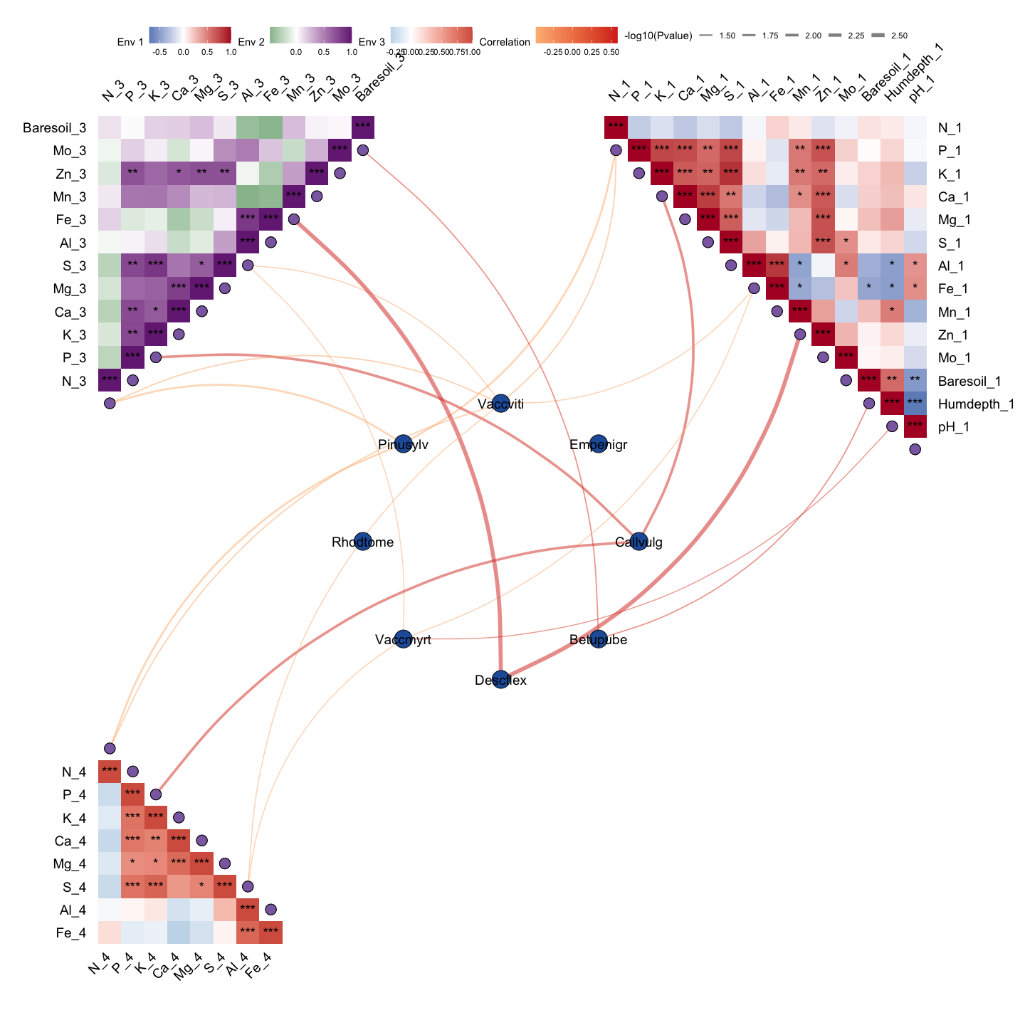
sessionInfo
sessionInfo()
#> R version 4.5.1 (2025-06-13)
#> Platform: aarch64-apple-darwin20
#> Running under: macOS Tahoe 26.2
#>
#> Matrix products: default
#> BLAS:   /Library/Frameworks/R.framework/Versions/4.5-arm64/Resources/lib/libRblas.0.dylib
#> LAPACK: /Library/Frameworks/R.framework/Versions/4.5-arm64/Resources/lib/libRlapack.dylib;  LAPACK version 3.12.1
#>
#> locale:
#> [1] en_US.UTF-8/en_US.UTF-8/en_US.UTF-8/C/en_US.UTF-8/en_US.UTF-8
#>
#> time zone: Asia/Shanghai
#> tzcode source: internal
#>
#> attached base packages:
#> [1] stats     graphics  grDevices utils     datasets  methods   base
#>
#> other attached packages:
#> [1] ggNetView_1.4.17 ggnewscale_0.5.2 ggplot2_4.0.2
#>
#> loaded via a namespace (and not attached):
#>  [1] psych_2.6.1           tidyselect_1.2.1      WGCNA_1.74
#>  [4] viridisLite_0.4.3     dplyr_1.2.0           farver_2.1.2
#>  [7] viridis_0.6.5         S7_0.2.1              ggraph_2.2.2
#> [10] fastmap_1.2.0         tweenr_2.0.3          digest_0.6.39
#> [13] rpart_4.1.24          lifecycle_1.0.5       cluster_2.1.8.1
#> [16] survival_3.8-3        magrittr_2.0.4        compiler_4.5.1
#> [19] rlang_1.1.7           Hmisc_5.2-5           tools_4.5.1
#> [22] igraph_2.2.2          utf8_1.2.6            yaml_2.3.12
#> [25] data.table_1.18.2.1   knitr_1.51            FNN_1.1.4.1
#> [28] labeling_0.4.3        graphlayouts_1.2.2    htmlwidgets_1.6.4
#> [31] mnormt_2.1.2          RColorBrewer_1.1-3    withr_3.0.2
#> [34] foreign_0.8-90        purrr_1.2.1           BiocGenerics_0.56.0
#> [37] nnet_7.3-20           dynamicTreeCut_1.63-1 grid_4.5.1
#> [40] polyclip_1.10-7       stats4_4.5.1          preprocessCore_1.70.0
#> [43] multtest_2.64.0       colorspace_2.1-2      fastcluster_1.3.0
#> [46] scales_1.4.0          iterators_1.0.14      MASS_7.3-65
#> [49] dichromat_2.0-0.1     cli_3.6.5             rmarkdown_2.30
#> [52] generics_0.1.4        otel_0.2.0            rstudioapi_0.18.0
#> [55] cachem_1.1.0          ggforce_0.5.0         stringr_1.6.0
#> [58] splines_4.5.1         parallel_4.5.1        impute_1.82.0
#> [61] matrixStats_1.5.0     base64enc_0.1-6       vctrs_0.7.1
#> [64] Matrix_1.7-4          ggrepel_0.9.6         Formula_1.2-5
#> [67] htmlTable_2.4.3       foreach_1.5.2         tidyr_1.3.2
#> [70] glue_1.8.0            codetools_0.2-20      stringi_1.8.7
#> [73] gtable_0.3.6          tibble_3.3.1          pillar_1.11.1
#> [76] htmltools_0.5.9       R6_2.6.1              doParallel_1.0.17
#> [79] tidygraph_1.3.1       evaluate_1.0.5        lattice_0.22-7
#> [82] Biobase_2.70.0        backports_1.5.0       memoise_2.0.1
#> [85] Rcpp_1.1.1            nlme_3.1-168          gridExtra_2.3
#> [88] checkmate_2.3.4       xfun_0.56             pkgconfig_2.0.3