8 Zi-Pi
Load R Package
library(tidyverse)   # data manipulation / piping utilities
library(ggNetView)   # graph builders + info-extraction helpers
Example data
# Access built-in example datasets in ggNetView

# ---- Dataset 1: Relative abundance table of rarefied ASVs/OTUs ----
# Rows = ASVs/OTUs (features / variables), Columns = samples
data("otu_rare_relative")
dim(otu_rare_relative)  # Check matrix dimensions: n_features x n_samples
## [1] 2859 18
otu_rare_relative[1:5, 1:5] # Preview first 5 rows x 5 cols to confirm data layout## KO1 KO2 KO3 KO4 KO5
## ASV_1 0.03306667 0.05453333 0.02013333 0.03613333 0.02686667
## ASV_2 0.05750000 0.03393333 0.06046667 0.05810000 0.07320000
## ASV_3 0.01733333 0.01296667 0.02290000 0.02336667 0.03106667
## ASV_4 0.04266667 0.01093333 0.01416667 0.01933333 0.03346667
## ASV_6 0.02646667 0.01856667 0.02110000 0.02353333 0.03806667
# ---- Dataset 2: Taxonomic annotation table for ASVs/OTUs ----
# Rows = ASVs/OTUs (row names should match the abundance table above)
# Columns = taxonomic ranks (Kingdom ~ Species, etc.)
data("tax_tab")
dim(tax_tab)
## [1] 2859 8
tax_tab[1:5, 1:5]## # A tibble: 5 × 5
## OTUID Kingdom Phylum Class Order
## <chr> <chr> <chr> <chr> <chr>
## 1 ASV_2 Archaea Thaumarchaeota Unassigned Nitrososphaerales
## 2 ASV_3 Bacteria Verrucomicrobia Spartobacteria Unassigned
## 3 ASV_31 Bacteria Actinobacteria Actinobacteria Actinomycetales
## 4 ASV_27 Archaea Thaumarchaeota Unassigned Nitrososphaerales
## 5 ASV_9 Bacteria Unassigned Unassigned UnassignedBuild graph object
# ---- Build a co-occurrence network from an abundance matrix ----
# Internal pipeline: transform -> correlation -> p-value adjustment ->
# edge filtering -> community detection -> attach taxonomy.
graph_obj <- build_graph_from_mat(
  mat              = otu_rare_relative,  # variables x samples numeric matrix
  transfrom.method = "none",             # input already relative abundance, no extra transform
  method           = "WGCNA",            # correlation backend: WGCNA::corAndPvalue
  proc             = "bonferroni",       # multiple-testing correction
  r.threshold      = 0.7,                # |r| cutoff for keeping an edge
  p.threshold      = 0.05,               # adjusted p-value cutoff
  node_annotation  = tax_tab,            # taxonomy joined onto each node by name
  top_modules      = 15,                 # keep top-15 modules; rest -> "Others"
  seed             = 1115                # fix RNG for reproducibility
)

graph_obj   # tbl_graph with Modularity / Degree / Strength + taxonomy columns
## # A tbl_graph: 213 nodes and 844 edges
## #
## # An undirected simple graph with 29 components
## #
## # Node Data: 213 × 14 (active)
## name modularity modularity2 modularity3 Modularity Degree Strength Kingdom
## <chr> <fct> <ord> <chr> <ord> <dbl> <dbl> <chr>
## 1 ASV_649 5 5 5 5 27 26.5 Bacter…
## 2 ASV_705 5 5 5 5 27 26.5 Bacter…
## 3 ASV_12… 5 5 5 5 27 26.5 Bacter…
## 4 ASV_13… 5 5 5 5 27 26.5 Bacter…
## 5 ASV_14… 5 5 5 5 27 26.5 Bacter…
## 6 ASV_14… 5 5 5 5 27 26.5 Bacter…
## 7 ASV_24… 5 5 5 5 27 26.5 Bacter…
## 8 ASV_25… 5 5 5 5 27 26.4 Bacter…
## 9 ASV_28… 5 5 5 5 27 26.5 Bacter…
## 10 ASV_28… 5 5 5 5 27 26.5 Bacter…
## # ℹ 203 more rows
## # ℹ 6 more variables: Phylum <chr>, Class <chr>, Order <chr>, Family <chr>,
## # Genus <chr>, Species <chr>
## #
## # Edge Data: 844 × 5
## from to weight correlation corr_direction
## <int> <int> <dbl> <dbl> <chr>
## 1 194 195 0.959 0.959 Positive
## 2 185 208 0.954 0.954 Positive
## 3 185 213 0.957 0.957 Positive
## # ℹ 841 more rowsExtract the two inputs Zi-Pi needs from graph object
nodes_bulk <- get_graph_nodes(graph_obj)      # node table (module + degree cols)
adj_mat    <- get_graph_adjacency(graph_obj)  # adjacency / correlation matrix
8.1 Zi-Pi analysis and plot
role_palette <- c(
  "Peripherals"  = "#377eb8",
  "Connectors"   = "#4daf4a",
  "Module hubs"  = "#e41a1c",
  "Network hubs" = "#ff7f00"
)

zp <- ggnetview_zipi(
  nodes_bulk     = nodes_bulk,    # node table: IDs in rownames or a `name` col
  z_bulk_mat     = adj_mat,       # adjacency matrix; non-zero entries = edges
  modularity_col = "Modularity",  # column holding module labels (no NAs)
  degree_col     = "Degree",      # column holding node degree   (no NAs)
  zi_threshold   = 2.5,           # Zi cutoff for role classification
  pi_threshold   = 0.62,          # Pi cutoff for role classification
  na.rm          = FALSE,         # FALSE = keep unclassifiable nodes (type = NA)
  point_colors   = role_palette,  # point + legend colours, keyed by role
  bg_colors      = c(             # quadrant background fills, keyed by role
    "Peripherals"  = "#f0f0f0",
    "Connectors"   = "#d9f0d3",
    "Module hubs"  = "#fde0dd",
    "Network hubs" = "#fee8c8"
  ),
  label_colors   = role_palette,  # quadrant text-label colours (default: black)
  label_size     = 5,             # quadrant text-label size  (default 5.5)
  bg_alpha       = 0.35           # background opacity 0..1    (default 0.25)
)


class(zp)
## [1] "list"
names(zp)## [1] "data" "plot"Output
zp$plot # the Zi-Pi quadrant plot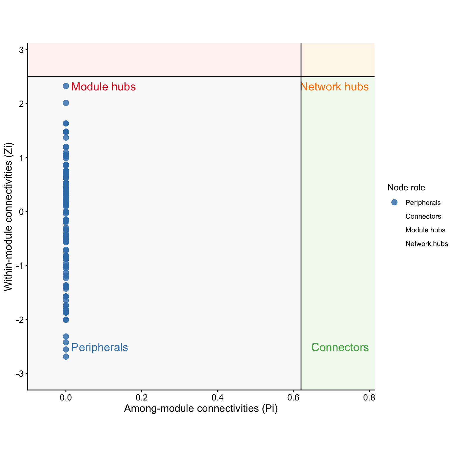
head(zp$data) # node table + Zi / Pi / type## name modularity modularity2 modularity3 Modularity Degree Strength
## 1 ASV_649 5 5 5 5 27 26.51226
## 2 ASV_705 5 5 5 5 27 26.46287
## 3 ASV_1234 5 5 5 5 27 26.45519
## 4 ASV_1373 5 5 5 5 27 26.51017
## 5 ASV_1479 5 5 5 5 27 26.49888
## 6 ASV_1481 5 5 5 5 27 26.51017
## Kingdom Phylum Class Order
## 1 Bacteria Proteobacteria Alphaproteobacteria Rhizobiales
## 2 Bacteria Actinobacteria Actinobacteria Actinomycetales
## 3 Bacteria Gemmatimonadetes Gemmatimonadetes Gemmatimonadales
## 4 Bacteria Actinobacteria Actinobacteria Solirubrobacterales
## 5 Bacteria Verrucomicrobia Spartobacteria Unassigned
## 6 Bacteria Proteobacteria Gammaproteobacteria Unassigned
## Family Genus
## 1 Unassigned Unassigned
## 2 Cellulomonadaceae Cellulomonas
## 3 Gemmatimonadaceae Gemmatimonas
## 4 Solirubrobacteraceae Solirubrobacter
## 5 Unassigned Spartobacteria_genera_incertae_sedis
## 6 Unassigned Unassigned
## Species within_module_connectivities
## 1 Unassigned 0.7566222
## 2 Cellulomonas_aerilata 0.7566222
## 3 Gemmatimonas_aurantiaca 0.7566222
## 4 Unassigned 0.7566222
## 5 Unassigned 0.7566222
## 6 Unassigned 0.7566222
## among_module_connectivities type
## 1 0 Peripherals
## 2 0 Peripherals
## 3 0 Peripherals
## 4 0 Peripherals
## 5 0 Peripherals
## 6 0 Peripherals
table(zp$data$type, useNA = "ifany") ##
## Peripherals Connectors Module hubs Network hubs
## 213 0 0 0Minimal call: only the required arguments
#  Minimal call: only the required arguments

zp_min <- ggnetview_zipi(
  nodes_bulk, adj_mat,
  modularity_col = "Modularity",
  degree_col     = "Degree"
)


# The three point_colors styles
zp_unnamed <- ggnetview_zipi(
  nodes_bulk, adj_mat, "Modularity", "Degree",
  point_colors = c("#1b9e77", "#d95f02", "#7570b3", "#e7298a")  # by fixed order
)

zp_named <- ggnetview_zipi(
  nodes_bulk, adj_mat, "Modularity", "Degree",
  point_colors = c("Network hubs" = "purple",                  # override a subset;
                   "Module hubs"  = "firebrick")               # others stay default
)

zp_single <- ggnetview_zipi(
  nodes_bulk, adj_mat, "Modularity", "Degree",
  point_colors = "steelblue"                                   # all four roles
)

# Background tweaks

zp_nobg <- ggnetview_zipi(
  nodes_bulk, adj_mat, "Modularity", "Degree",
  bg_alpha = 0                       # disable quadrant shading entirely
)
final_plot <- zp$plot +
  labs(title = "Zi-Pi topological roles") +
  theme(legend.position = "bottom")

final_plot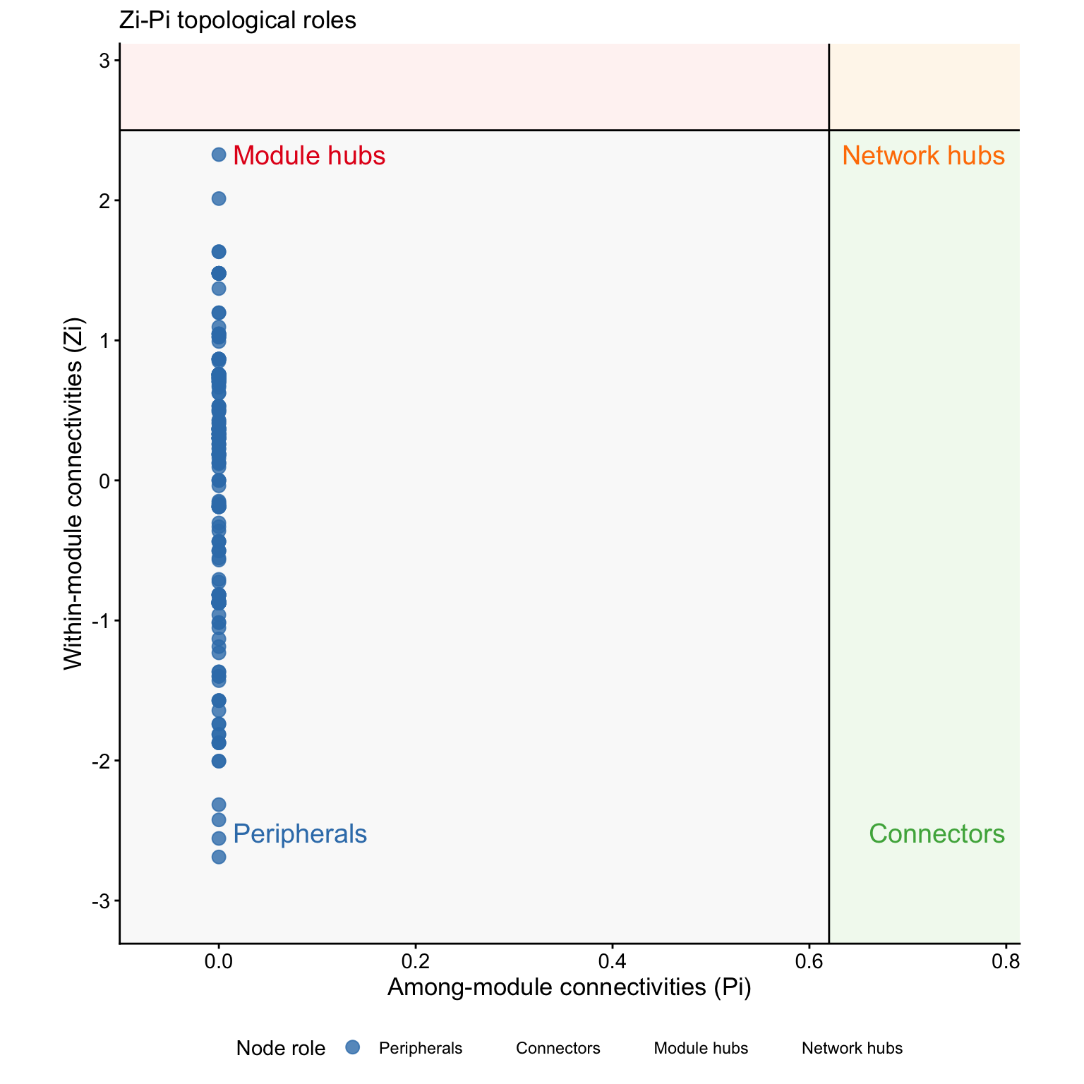
# ggsave("zipi_demo.pdf", final_plot, width = 6, height = 6) # square fits aspect.ratio = 1
# Pull out the most structurally important nodes (Network hubs):
subset(
  zp$data,
  type == "Network hubs",
  select = c(name, type, within_module_connectivities, among_module_connectivities)
)
## [1] name type
## [3] within_module_connectivities among_module_connectivities
## <0 rows> (or 0-length row.names)