12 Gallery of Reproducible Examples
Load R Package
library(tidyverse)   # data manipulation / piping utilities
library(ggNetView)   # graph builders + info-extraction helpers
12.1 Microbial Community Network
The data from
Liu, X., Wang, M., Liu, B. et al. Keystone taxa mediate the trade-off between microbial community stability and performance in activated sludges. Nat Water 3, 723–733 (2025).DOI:10.1038/s44221-025-00451-6
# Load data

# OTU table: read the pre-filtered ASV abundance data (relative abundance range 0.00001-0.01)
# Use read_delim() to read the CSV file, and convert the first column ("...1") to row names
otu <- read_delim(file = "./Input/Figure3a-b_ASV_data_0.00001_0.01.csv", delim = ",", col_names = T) %>%
  tibble::column_to_rownames(var = "...1")

# OTU taxonomy table: read the ASV annotation information from the MiDAS database,
# including taxonomy, Mean Relative Abundance (MRA), and functional annotations.
# This table will be used to annotate the network nodes (e.g. by Phylum).
tax <- read_delim(file = "./Input/Figure3a-b_ASV-MiDAS-MRA-function-taxonomy-all-new.csv", col_names = T, delim = ",")

# Build the network graph object
# build_graph_from_mat() computes pairwise correlations among taxa from the OTU abundance matrix
# and constructs a network graph object for downstream visualization.
obj <- build_graph_from_mat(
  mat              = otu,        # input OTU abundance matrix
  transfrom.method = "ln",       # data transformation method: natural log (stabilize variance)
  method           = "WGCNA",    # correlation method: WGCNA (weighted gene co-expression network)
  r.threshold      = 0.44,       # correlation coefficient threshold: keep edges with |r| >= 0.44
  p.threshold      = 0.05,       # significance threshold: keep edges with p < 0.05
  node_annotation  = tax         # node annotation table providing taxonomic info for each node
)


# ====== Figure 1: network plot colored by Modularity (module assignment) ======
p1 <- ggNetView(
  graph_obj     = obj,           # input network graph object
  layout        = "gephi",       # layout algorithm: Gephi-style (ForceAtlas2-like)
  layout.module = "adjacent",    # module layout: place adjacent modules close together
  group.by      = "Modularity",  # grouping variable: color nodes by module ID
  center        = F,             # do not center the network
  jitter        = TRUE,          # add small random offsets to node positions to avoid overlap
  jitter_sd     = 0.15,          # standard deviation of the jitter
  shrink        = 0.9,           # shrink factor: tighten nodes within each module
  linealpha     = 0.2,           # transparency of edges
  linecolor     = "#d9d9d9"      # default edge color: light grey
) +
  # Manually assign fill colors for the 16 modules
  scale_fill_manual(values = c("#00A9FF", "#0BB702", "#C77CFF", "#00C19A", "#ED68ED",
                               "#8494FF", "#00B8E7", "#FF61CC", "#F8766D", "#E68613",
                               "#ABA300", "#7CAE00", "#CD9600", "#00BE67", "#00BFC4",
                               "#FF68A1")) +
  theme(legend.position = "none")    # remove legend

# Save Figure 1 as a PDF (commented out; uncomment to enable saving)
# ggsave(filename = "Figure3a-b/Figure3a.pdf",
#        plot     = p1,
#        height   = 12,
#        width    = 12)

p1   # display Figure 1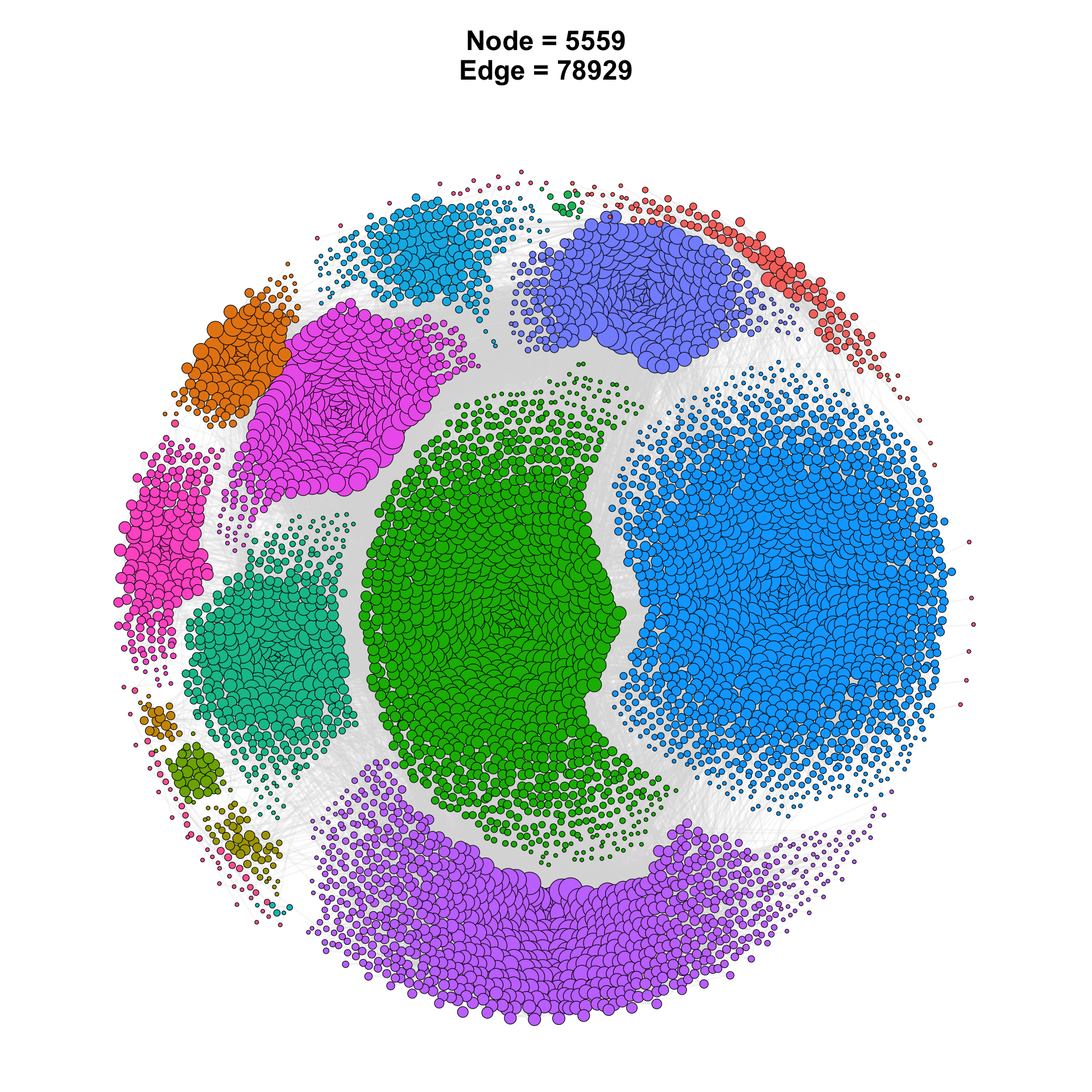
# ====== Figure 2: add  outlier ======

module_colors <- c("#00A9FF", "#0BB702", "#C77CFF", "#00C19A", "#ED68ED",
                   "#8494FF", "#00B8E7", "#FF61CC", "#F8766D", "#E68613",
                   "#ABA300", "#7CAE00", "#CD9600", "#00BE67", "#00BFC4",
                   "#FF68A1")

p2 <- ggNetView(
  graph_obj        = obj,             # input network graph object
  layout           = "gephi",         # layout algorithm: Gephi-style (ForceAtlas2-like)
  layout.module    = "adjacent",      # module layout: place adjacent modules close together
  group.by         = "Modularity",    # grouping variable: color nodes by module ID
  center           = F,               # do not force a node at the layout centre
  pointalpha       = 0.5,             # node transparency (0 = invisible, 1 = opaque)
  label            = T,               # draw module text labels
  label_layout     = "two_column",    # label_layout defaults to "two_column": labels are placed in two fixed
  label_wrap_width = 18,              # wrap long module / pathway names at ~18 chars per line
  label_outer_pad  = 0.25,            # distance from the network edge to each label column
  jitter           = TRUE,            # add small random offsets to node positions
  jitter_sd        = 0.15,            # standard deviation of the jitter
  shrink           = 0.9,             # shrink factor: tighten nodes within each module
  linealpha        = 0.2,             # transparency of edges
  linecolor        = "#d9d9d9",       # default edge colour: light grey
  add_outer        = T,               # add per-module outer boundary (KDE/HDR contour)
  outeralpha       = 0.3,             # per-module boundary fill transparency
  outerwidth       = 1,               # per-module boundary line width
  add_group_outer  = T,               # add an outer circle around the whole network
  fill             = module_colors,   # <-- node fill colours; module outers use the same palette
  color            = module_colors    # <-- module boundary line colours (matches the fills)
) +
  theme(legend.position = "none")     # hide all legends


# Save Figure 2 as a PDF (commented out; uncomment to enable saving)
# ggsave(filename = "Figure2.pdf",
#        plot     = p2,
#        height   = 12,
#        width    = 12)

p2   # display Figure 2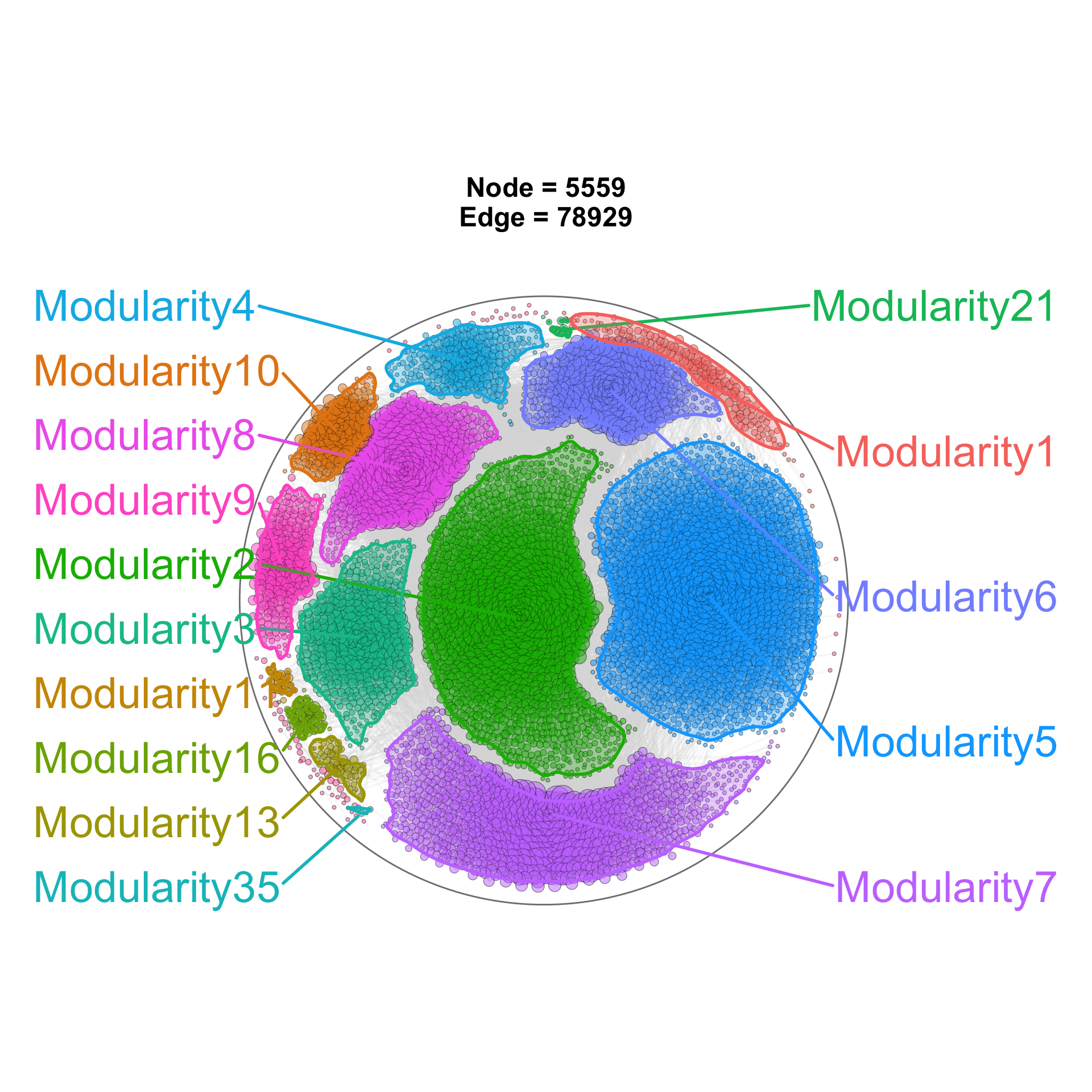
# ====== Figure 3: add  outlier ======

module_colors <- c("#00A9FF", "#0BB702", "#C77CFF", "#00C19A", "#ED68ED",
                   "#8494FF", "#00B8E7", "#FF61CC", "#F8766D", "#E68613",
                   "#ABA300", "#7CAE00", "#CD9600", "#00BE67", "#00BFC4",
                   "#FF68A1")

p3 <- ggNetView(
  graph_obj        = obj,             # input network graph object
  layout           = "gephi",         # layout algorithm: Gephi-style (ForceAtlas2-like)
  layout.module    = "adjacent",      # module layout: place adjacent modules close together
  group.by         = "Modularity",    # grouping variable: color nodes by module ID
  center           = F,               # do not force a node at the layout centre
  pointalpha       = 0.5,             # node transparency (0 = invisible, 1 = opaque)
  label            = T,               # draw module text labels
  label_layout     = "two_column_follow", # "two_column_follow": ring layout that follows each module's real
  label_wrap_width = 18,              # wrap long module / pathway names at ~18 chars per line
  label_outer_pad  = 0.25,            # outer ellipse padding: how far labels sit beyond the network
  jitter           = TRUE,            # add small random offsets to node positions
  jitter_sd        = 0.15,            # standard deviation of the jitter
  shrink           = 0.9,             # shrink factor: tighten nodes within each module
  linealpha        = 0.2,             # transparency of edges
  linecolor        = "#d9d9d9",       # default edge colour: light grey
  add_outer        = T,               # add per-module outer boundary (KDE/HDR contour)
  bandwidth_scale  = 2.0,             # KDE bandwidth multiplier; >1 -> smoother / rounder boundary
  outeralpha       = 0.3,             # per-module boundary fill transparency
  outerwidth       = 1,               # per-module boundary line width
  add_group_outer  = T,               # add an outer circle around the whole network
  fill             = module_colors,   # <-- node fill colours; module outers use the same palette
  color            = module_colors,   # <-- module boundary line colours (matches the fills)
  remove           = T,               # drop the "Others" module from rendering (keep layout intact)
  mapping_line     = T                # colour edges by their sign / weight category
                                      # (e.g. positive vs negative correlations get different colours)
) +
  theme(legend.position = "none")     # hide all legends


# Save Figure 3 as a PDF (commented out; uncomment to enable saving)
# ggsave(filename = "Figure3.pdf",
#        plot     = p3,
#        height   = 12,
#        width    = 12)

p3   # display Figure 3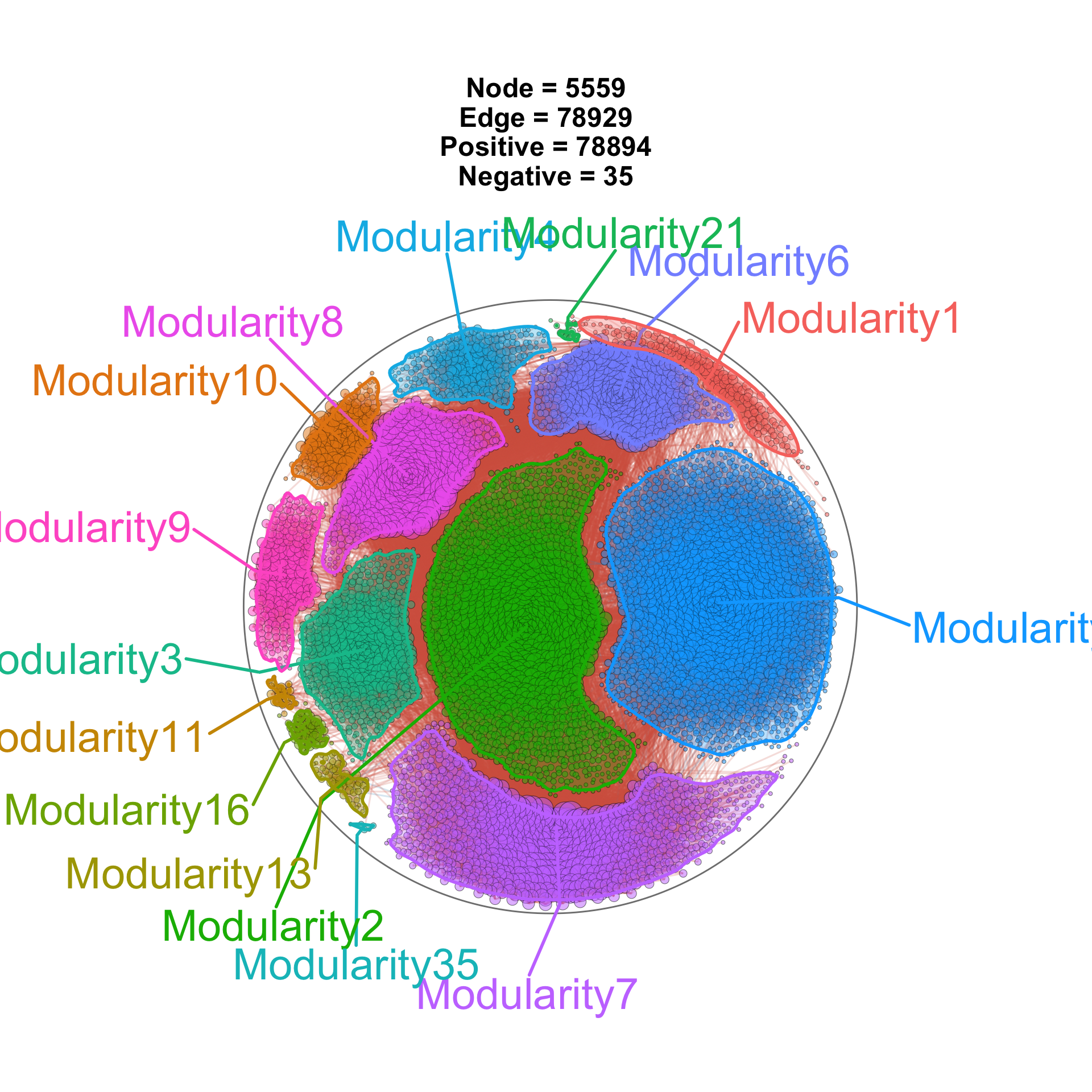
# ====== Figure 4: add  outlier ======

p4 <- ggNetView(
  graph_obj        = obj,             # input network graph object
  layout           = "gephi",         # layout algorithm: Gephi-style (ForceAtlas2-like)
  layout.module    = "adjacent",      # module layout: place adjacent modules close together
  group.by         = "Modularity",    # grouping variable: color nodes by module ID
  center           = F,               # do not force a node at the layout centre
  pointalpha       = 0.5,             # node transparency (0 = invisible, 1 = opaque)
  label            = T,               # draw module text labels
  label_layout     = "label_circle",  # "label_circle" ring layout that follows each module's real angular
  label_wrap_width = 18,              # wrap long module / pathway names at ~18 chars per line
  label_outer_pad  = 0.25,            # outer ellipse padding: how far labels sit beyond the network
  jitter           = TRUE,            # add small random offsets to node positions
  jitter_sd        = 0.15,            # standard deviation of the jitter
  shrink           = 0.9,             # shrink factor: tighten nodes within each module
  linealpha        = 0.2,             # transparency of edges
  linecolor        = "#d9d9d9",       # default edge colour: light grey
  add_outer        = T,               # add per-module outer boundary (KDE/HDR contour)
  outeralpha       = 0.3,             # per-module boundary fill transparency
  outerwidth       = 1,               # per-module boundary line width
  add_group_outer  = T,               # add an outer circle around the whole network
  fill             = module_colors,   # <-- node fill colours; module outers use the same palette
  color            = module_colors    # <-- module boundary line colours (matches the fills)
) +
  theme(legend.position = "none")     # hide all legends


# Save Figure 4 as a PDF (commented out; uncomment to enable saving)
# ggsave(filename = "Figure4.pdf",
#        plot     = p4,
#        height   = 12,
#        width    = 12)

p4   # display Figure 4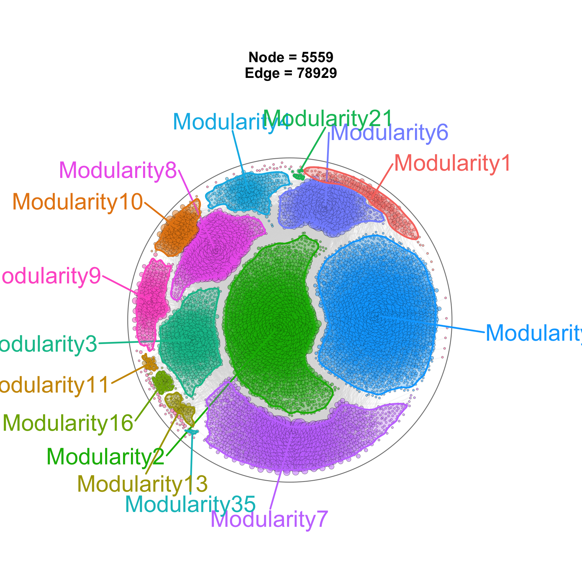
# ====== Figure 5: network plot colored by Phylum, with positive/negative edges mapped ======
p5 <- ggNetView(
  graph_obj     = obj,           # input the same network graph object
  layout        = "gephi",       # layout algorithm: Gephi-style
  layout.module = "adjacent",    # adjacent module layout
  fill.by       = "Phylum",      # grouping variable: color nodes by Phylum
  center        = F,             # do not center the network
  jitter        = TRUE,          # add jitter to node positions
  jitter_sd     = 0.15,          # jitter standard deviation
  mapping_line  = TRUE,          # map edge color by correlation sign (positive / negative)
  shrink        = 0.9,           # shrink factor for modules
  linealpha     = 0.2,           # edge transparency
  linecolor     = "#d9d9d9"      # default edge color (overridden when mapping_line = TRUE)
) +
  # Manually assign fill colors for Phylum: a soft palette repeated 3 times to cover many phyla
  scale_fill_manual(values = rep(c("#8dd3c7",
                                   "#ffffb3", "#bebada", "#fb8072", "#80b1d3",
                                   "#fdb462", "#b3de69", "#fccde5", "#cab2d6",
                                   "#bc80bd", "#ccebc5", "#ffed6f", "#a6cee3",
                                   "#b2df8a", "#fb9a99", "#bdbdbd", "#a6cee3",
                                   "#1f78b4", "#b2df8a", "#33a02c", "#fb9a99",
                                   "#e31a1c", "#fdbf6f", "#ff7f00", "#cab2d6",
                                   "#6a3d9a", "#ffff99", "#b15928"), times = 3)) +
  # Edge colors: red for positive correlations, blue for negative correlations
  scale_color_manual(values = c("Positive" = "#d6604d",
                                "Negative" = "#92c5de")) +
  scale_size(range = c(1, 5)) +      # map node size to the range [1, 5]
  theme(legend.position = "none")    # remove legend

# Save Figure 5 as a PDF (commented out; uncomment to enable saving)
# ggsave(filename = "Figure5.pdf",
#        plot     = p5,
#        height   = 12,
#        width    = 12)

p5   # display Figure 5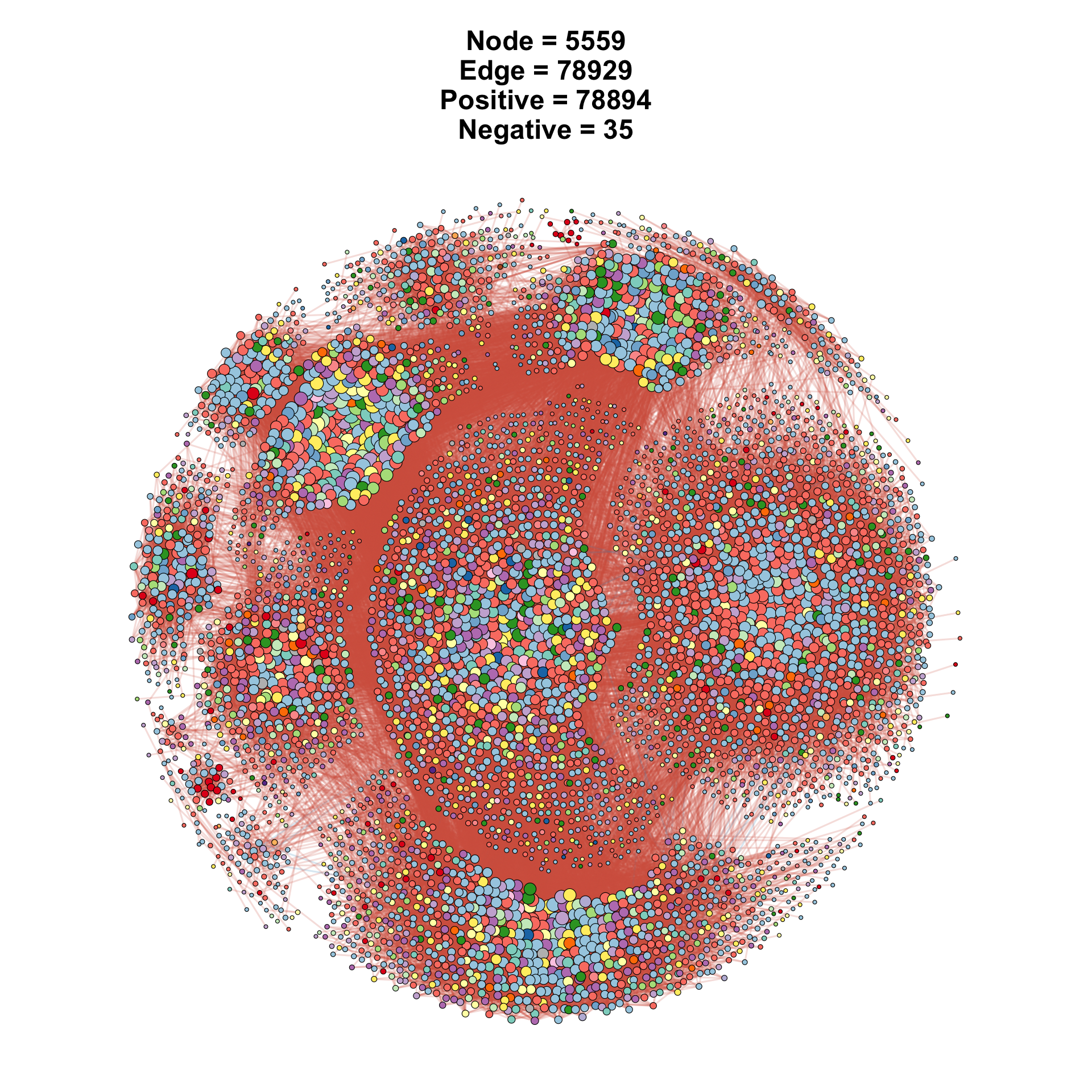
12.2 WGCNA network
load(file = "./Input/WGCNA.tom-block.1.RData")
TOM_mat <- as.matrix(TOM)

plot.mat = readRDS(file = "./Input/plot.mat.Rds")

trans_TOM <- trans_TOM_in_WGCNA(TOM_mat, plot.mat, top_k = 1)

net <- readRDS(file = "./Input/net.Rds")

module <- data.frame(
  ID = names(net$colors),
  Module = as.character(net$colors)
)

id <- data.frame(
  ID = names(sort(net$colors))
)

obj <- build_graph_from_wgcna(
  wgcna_tom = trans_TOM,
  module = module,
  node_annotation = id
)

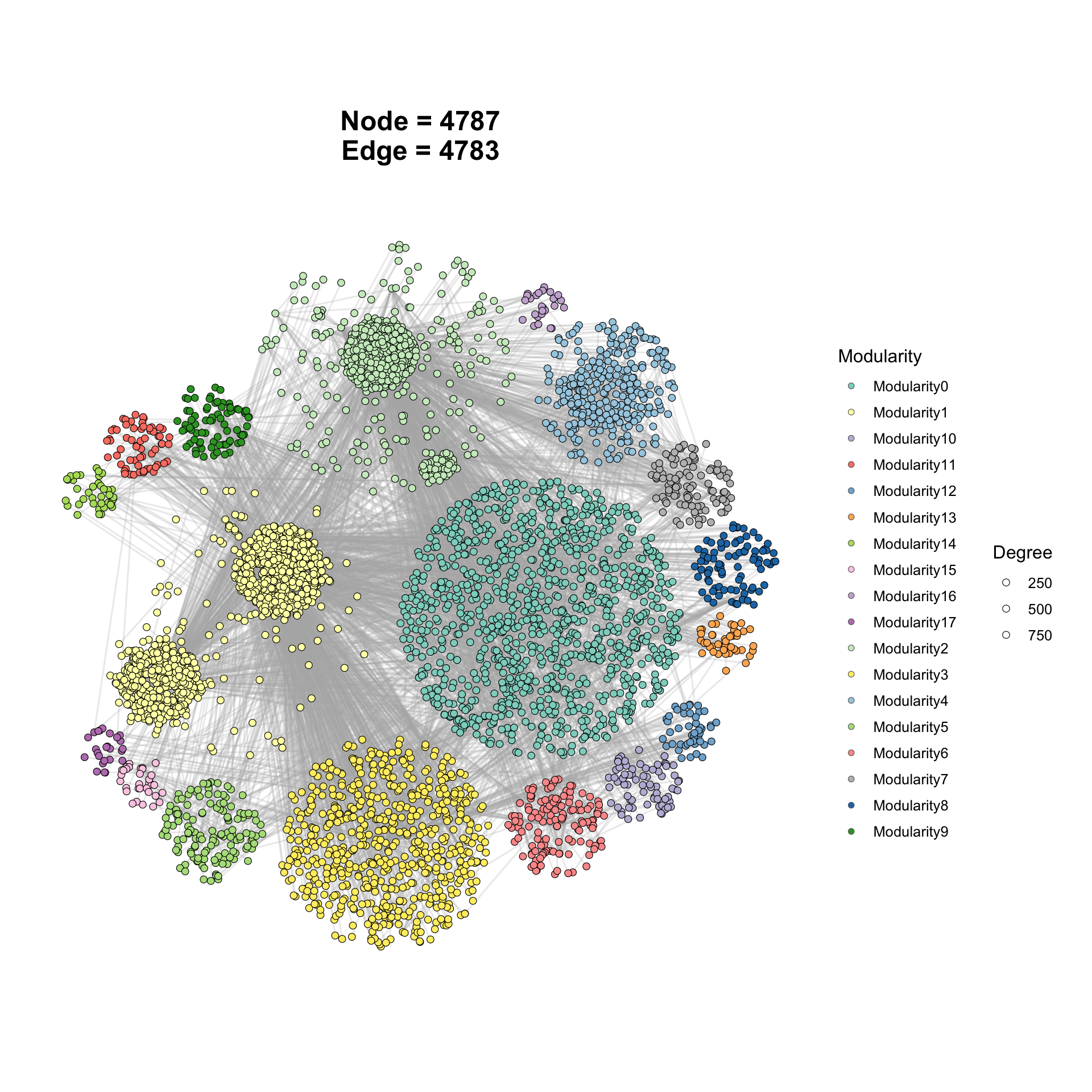
obj
## # A tbl_graph: 4787 nodes and 4783 edges
## #
## # An unrooted forest with 4 trees
## #
## # Node Data: 4,787 × 8 (active)
## name Module modularity modularity2 modularity3 Modularity Degree Strength
## <chr> <chr> <fct> <fct> <chr> <fct> <dbl> <dbl>
## 1 HBA1_41… 0 0 0 0 0 5 0.578
## 2 HBB_4169 0 0 0 0 0 4 0.507
## 3 CA1_3480 0 0 0 0 0 3 0.360
## 4 PMP2_15… 0 0 0 0 0 2 0.162
## 5 ZC3HAV1… 0 0 0 0 0 2 0.0755
## 6 RGS10_5 0 0 0 0 0 1 0.172
## 7 ITGA2B_7 0 0 0 0 0 1 0.134
## 8 MARK3_9 0 0 0 0 0 1 0.0957
## 9 PTPRJ_10 0 0 0 0 0 1 0.0227
## 10 THOC5_11 0 0 0 0 0 1 0.0447
## # ℹ 4,777 more rows
## #
## # Edge Data: 4,783 × 3
## from to weight
## <int> <int> <dbl>
## 1 121 1075 0.145
## 2 1075 1272 0.246
## 3 93 1066 0.132
## # ℹ 4,780 more rows
p <- ggNetView(
  graph_obj = obj,
  layout = "WGCNA",  # 使用 WGCNA 布局
  layout.module = "order",  # 或其他选项
  group.by = "Modularity",
  fill.by = "Modularity",
  center = F,
  shrink = 0.95,
  jitter = F,
  jitter_sd = 1.5,
  pointsize = c(2,2),
  seed = 1
)

p