6 Network layout
Load R Package
library(tidyverse)   # data manipulation / piping utilities
library(ggNetView)   # graph builders + layout/plotting frontend
Example data
# ---- Built-in example datasets ----

# Relative abundance table of rarefied ASVs/OTUs (rows = ASVs, cols = samples).
data("otu_rare_relative")
dim(otu_rare_relative)
## [1] 2859 18
otu_rare_relative[1:5, 1:5]## KO1 KO2 KO3 KO4 KO5
## ASV_1 0.03306667 0.05453333 0.02013333 0.03613333 0.02686667
## ASV_2 0.05750000 0.03393333 0.06046667 0.05810000 0.07320000
## ASV_3 0.01733333 0.01296667 0.02290000 0.02336667 0.03106667
## ASV_4 0.04266667 0.01093333 0.01416667 0.01933333 0.03346667
## ASV_6 0.02646667 0.01856667 0.02110000 0.02353333 0.03806667## [1] 2859 8
tax_tab[1:5, 1:5]## # A tibble: 5 × 5
## OTUID Kingdom Phylum Class Order
## <chr> <chr> <chr> <chr> <chr>
## 1 ASV_2 Archaea Thaumarchaeota Unassigned Nitrososphaerales
## 2 ASV_3 Bacteria Verrucomicrobia Spartobacteria Unassigned
## 3 ASV_31 Bacteria Actinobacteria Actinobacteria Actinomycetales
## 4 ASV_27 Archaea Thaumarchaeota Unassigned Nitrososphaerales
## 5 ASV_9 Bacteria Unassigned Unassigned UnassignedBuild graph object
# ---- Build a co-occurrence network used by every layout demo below ----
graph_obj <- build_graph_from_mat(
  mat              = otu_rare_relative,  # variables x samples numeric matrix
  transfrom.method = "none",             # already relative abundance, no extra transform
  r.threshold      = 0.7,                # |r| cutoff for keeping an edge
  p.threshold      = 0.05,               # adjusted p-value cutoff
  method           = "WGCNA",            # correlation backend: WGCNA::corAndPvalue
  cor.method       = "pearson",          # Pearson correlation
  proc             = "BH",               # multiple-testing correction (Benjamini-Hochberg)
  module.method    = "Fast_greedy",      # community detection algorithm
  node_annotation  = tax_tab,            # taxonomy joined onto nodes by name
  top_modules      = 15,                 # keep top-15 modules; rest -> "Others"
  seed             = 1115                # fix RNG for reproducibility
)

graph_obj
## # A tbl_graph: 2049 nodes and 9602 edges
## #
## # An undirected simple graph with 100 components
## #
## # Node Data: 2,049 × 14 (active)
## name modularity modularity2 modularity3 Modularity Degree Strength Kingdom
## <chr> <fct> <ord> <chr> <ord> <dbl> <dbl> <chr>
## 1 ASV_916 1 1 1 1 58 50.5 Bacter…
## 2 ASV_777 1 1 1 1 58 48.7 Bacter…
## 3 ASV_606 1 1 1 1 55 45.8 Bacter…
## 4 ASV_740 1 1 1 1 54 47.2 Bacter…
## 5 ASV_14… 1 1 1 1 54 44.5 Bacter…
## 6 ASV_23… 1 1 1 1 54 47.4 Bacter…
## 7 ASV_15… 1 1 1 1 52 45.3 Bacter…
## 8 ASV_24… 1 1 1 1 52 43.0 Bacter…
## 9 ASV_19… 1 1 1 1 52 43.0 Bacter…
## 10 ASV_568 1 1 1 1 51 45.1 Bacter…
## # ℹ 2,039 more rows
## # ℹ 6 more variables: Phylum <chr>, Class <chr>, Order <chr>, Family <chr>,
## # Genus <chr>, Species <chr>
## #
## # Edge Data: 9,602 × 5
## from to weight correlation corr_direction
## <int> <int> <dbl> <dbl> <chr>
## 1 1771 1825 0.793 0.793 Positive
## 2 594 597 0.895 0.895 Positive
## 3 588 597 0.864 0.864 Positive
## # ℹ 9,599 more rows6.1 Full graph layout
6.1.1 Gephi layout
layout.module = “random”
# Gephi-style ForceAtlas2-like layout: good general-purpose layout for
# scale-free / community-rich biological networks.
p <- ggNetView(
  graph_obj     = graph_obj,    # the tbl_graph to draw
  layout        = "gephi",      # global node-positioning algorithm
  center        = F,            # don't pull all modules toward the plot center
  shrink        = 0.8,          # scale each module inward (smaller = tighter modules)
  layout.module = "random",     # how modules are placed relative to each other: "random" / "adjacent" / "order"
  group.by      = "Modularity", # grouping variable used for per-module layout
  fill.by       = "Modularity"  # node fill colour mapped to module ID
)

p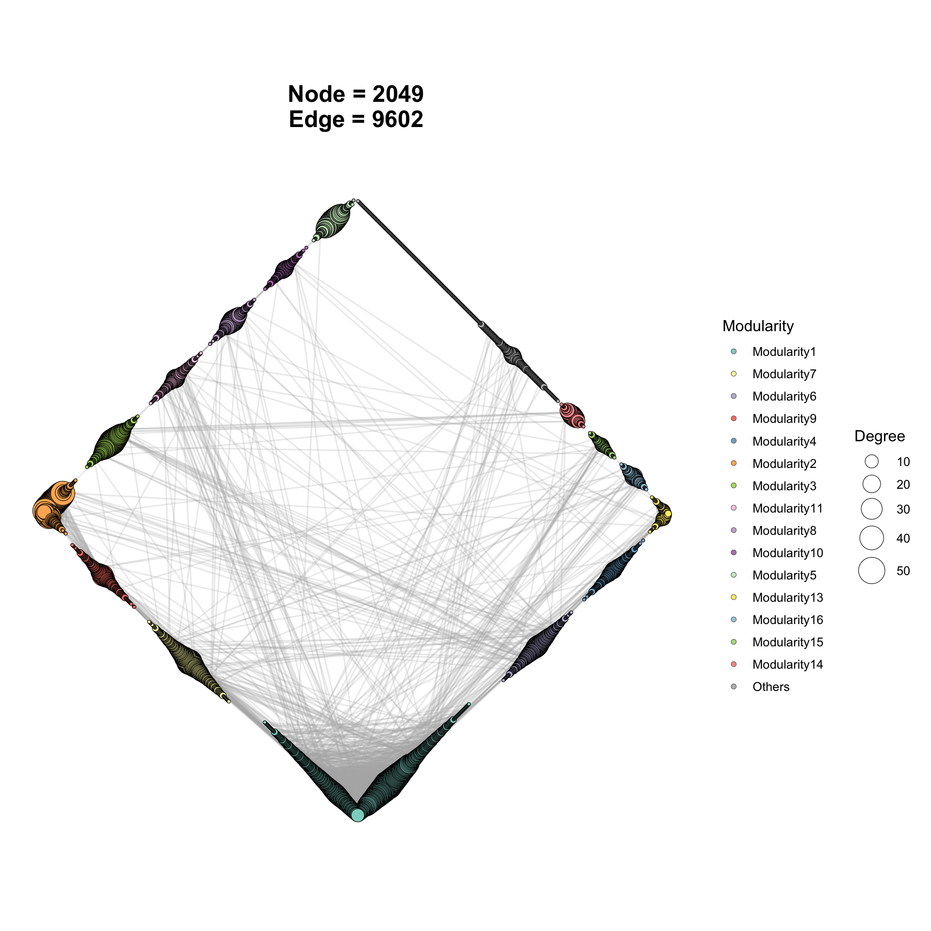
layout.module = “adjacent”
# Gephi-style ForceAtlas2-like layout: good general-purpose layout for
# scale-free / community-rich biological networks.
p <- ggNetView(
  graph_obj     = graph_obj,    # the tbl_graph to draw
  layout        = "gephi",      # global node-positioning algorithm
  center        = F,            # don't pull all modules toward the plot center
  shrink        = 0.8,          # scale each module inward (smaller = tighter modules)
  layout.module = "adjacent",     # how modules are placed relative to each other: "random" / "adjacent" / "order"
  group.by      = "Modularity", # grouping variable used for per-module layout
  fill.by       = "Modularity"  # node fill colour mapped to module ID
)

p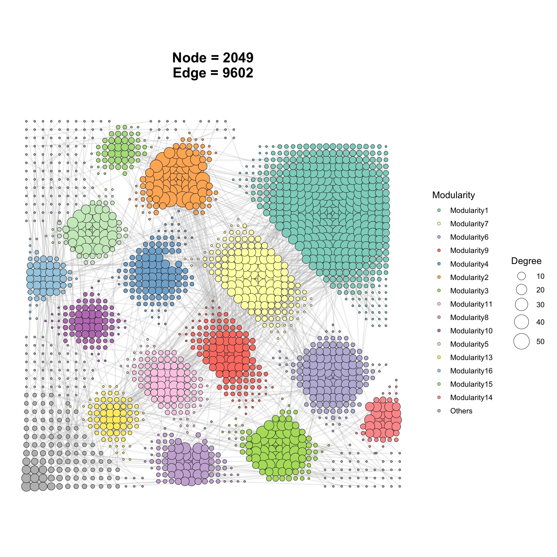
layout.module = “order”
# Gephi-style ForceAtlas2-like layout: good general-purpose layout for
# scale-free / community-rich biological networks.
p <- ggNetView(
  graph_obj     = graph_obj,    # the tbl_graph to draw
  layout        = "gephi",      # global node-positioning algorithm
  center        = F,            # don't pull all modules toward the plot center
  shrink        = 1,          # scale each module inward (smaller = tighter modules)
  layout.module = "order",     # how modules are placed relative to each other: "random" / "adjacent" / "order"
  group.by      = "Modularity", # grouping variable used for per-module layout
  fill.by       = "Modularity"  # node fill colour mapped to module ID
)

p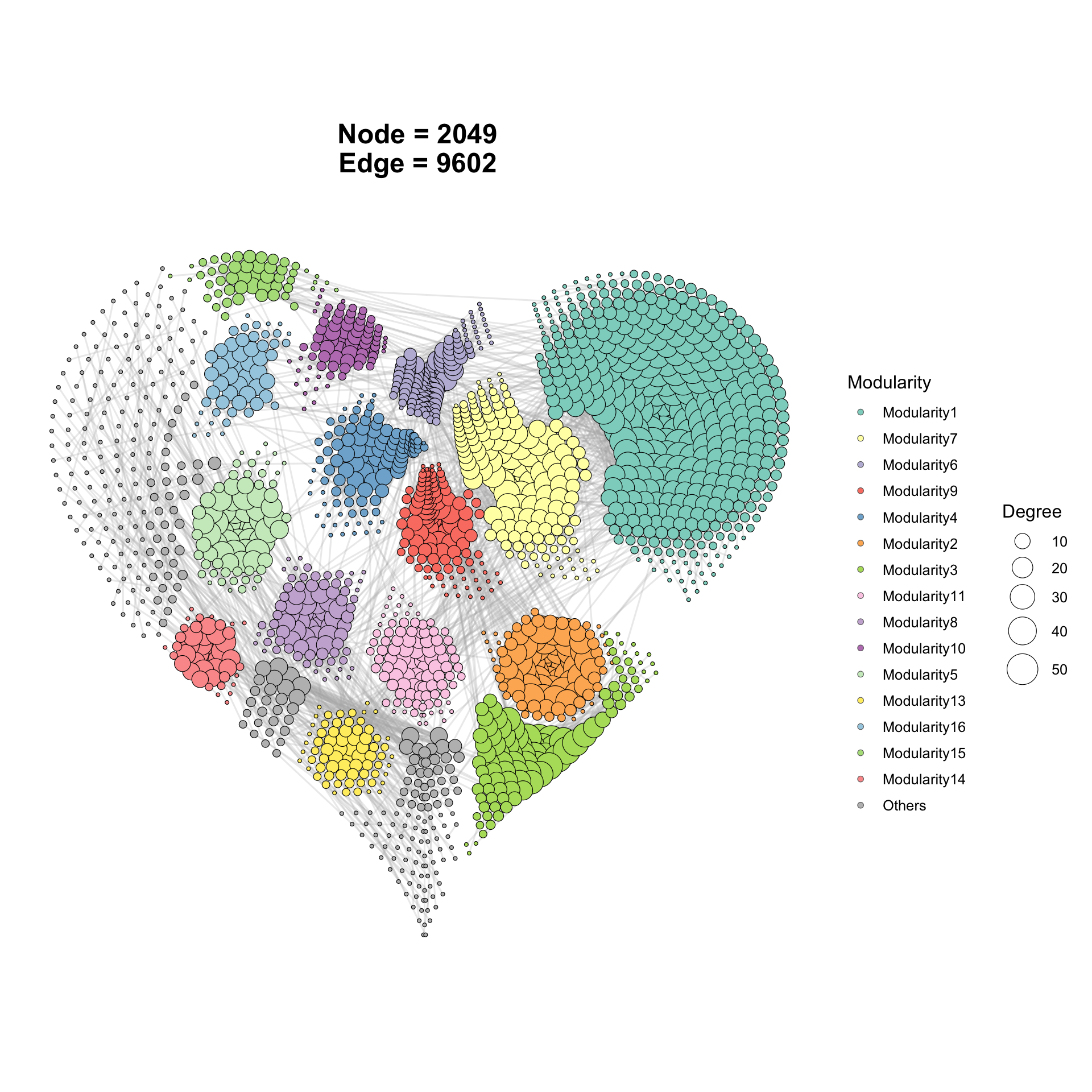
6.1.2 Fruchterman–Reingold force-directed layout
# FR2: a force-directed layout (springs pull connected nodes, repulsion pushes
# all others apart). Classic choice; reveals dense vs. sparse regions clearly.
p <- ggNetView(
  graph_obj     = graph_obj,
  layout        = "fr2",        # Fruchterman-Reingold variant
  center        = F,
  shrink        = 0.8,
  layout.module = "random",     # modules placed independently from each other
  group.by      = "Modularity",
  fill.by       = "Modularity"
)

p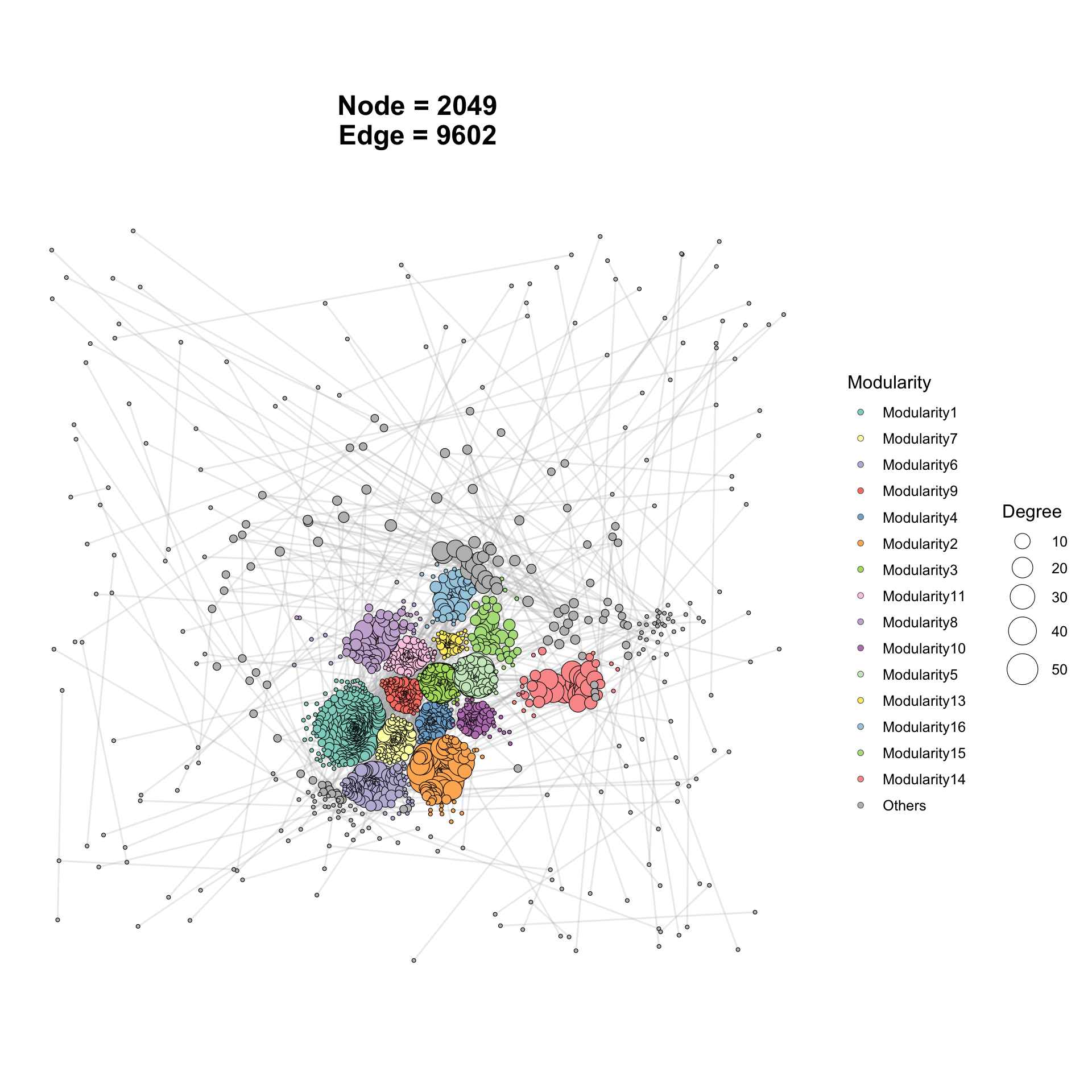
6.1.3 Diamond layout
# "diamond": modules arranged on a rhombic / diamond-shaped lattice.
# Good for showing many modules side-by-side without overlap.
p <- ggNetView(
  graph_obj     = graph_obj,
  layout        = "diamond",
  center        = F,
  shrink        = 0.8,
  layout.module = "adjacent",   # neighbouring modules placed close together to minimise gaps
  group.by      = "Modularity",
  fill.by       = "Modularity"
)

p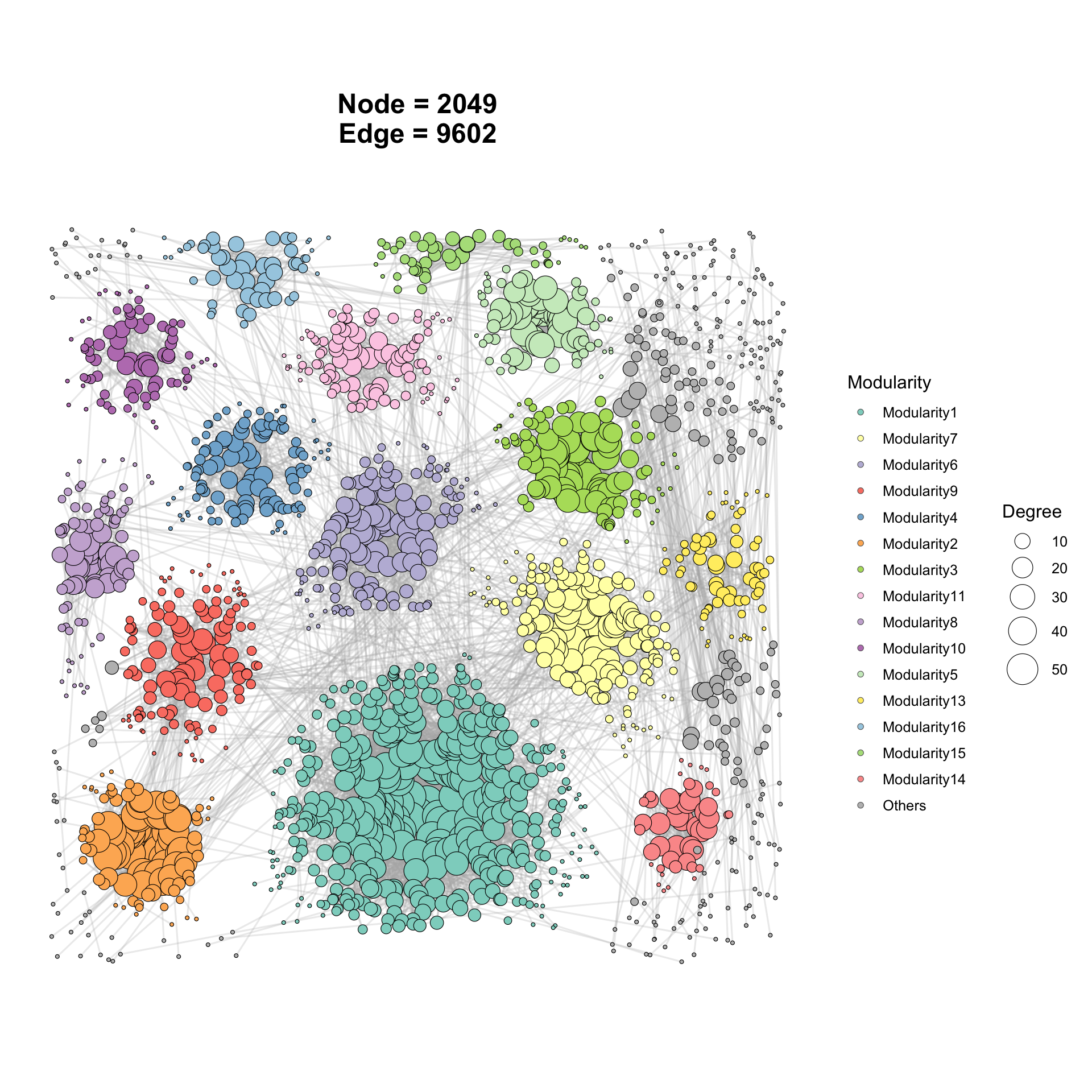
6.1.4 KK layout
# Kamada-Kawai force-directed layout: like FR but optimises a stress function;
# tends to give smoother, more even spacing for medium-sized networks.
p <- ggNetView(
  graph_obj     = graph_obj,
  layout        = "kk",
  center        = F,
  shrink        = 0.8,
  layout.module = "adjacent",
  group.by      = "Modularity",
  fill.by       = "Modularity"
)

p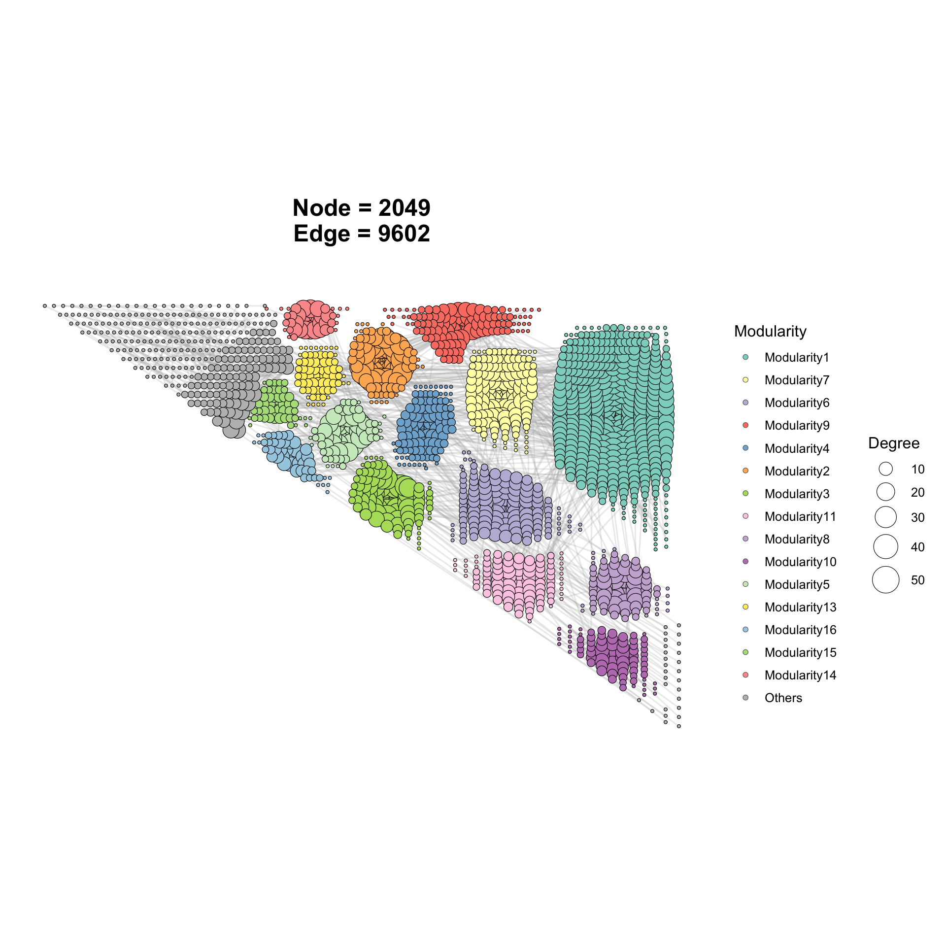
6.1.5 Nicley layout
# "nicely": igraph's auto-pick layout — chooses a reasonable algorithm based on
# graph size and structure. Safe default when you don't want to pick yourself.
p <- ggNetView(
  graph_obj     = graph_obj,
  layout        = "nicely",
  center        = F,
  shrink        = 0.8,
  layout.module = "adjacent",
  group.by      = "Modularity",
  fill.by       = "Modularity"
)
## Warning in ggNetView(graph_obj = graph_obj, layout = "nicely", center = F, :
## `layout.module = 'adjacent'` failed at k_nn = 12; retrying with k_nn = 32.## Warning in ggNetView(graph_obj = graph_obj, layout = "nicely", center = F, :
## `layout.module = 'adjacent'` failed at k_nn = 32; retrying with k_nn = 52.## Warning in ggNetView(graph_obj = graph_obj, layout = "nicely", center = F, :
## `layout.module = 'adjacent'` failed at k_nn = 52; retrying with k_nn = 72.## Warning in ggNetView(graph_obj = graph_obj, layout = "nicely", center = F, :
## `layout.module = 'adjacent'` failed at k_nn = 72; retrying with k_nn = 92.## Warning in ggNetView(graph_obj = graph_obj, layout = "nicely", center = F, :
## `layout.module = 'adjacent'` failed at k_nn = 92; retrying with k_nn = 115.## Warning in ggNetView(graph_obj = graph_obj, layout = "nicely", center = F, :
## `layout.module = 'adjacent'` failed at k_nn = 115; retrying with k_nn = 144.## Warning in ggNetView(graph_obj = graph_obj, layout = "nicely", center = F, :
## `layout.module = 'adjacent'` failed at k_nn = 144; retrying with k_nn = 180.## Warning in ggNetView(graph_obj = graph_obj, layout = "nicely", center = F, :
## `layout.module = 'adjacent'` failed at k_nn = 180; retrying with k_nn = 225.## Warning in ggNetView(graph_obj = graph_obj, layout = "nicely", center = F, :
## `layout.module = 'adjacent'` failed at k_nn = 225; retrying with k_nn = 282.## Warning in ggNetView(graph_obj = graph_obj, layout = "nicely", center = F, :
## `layout.module = 'adjacent'` failed at k_nn = 282; retrying with k_nn = 353.
p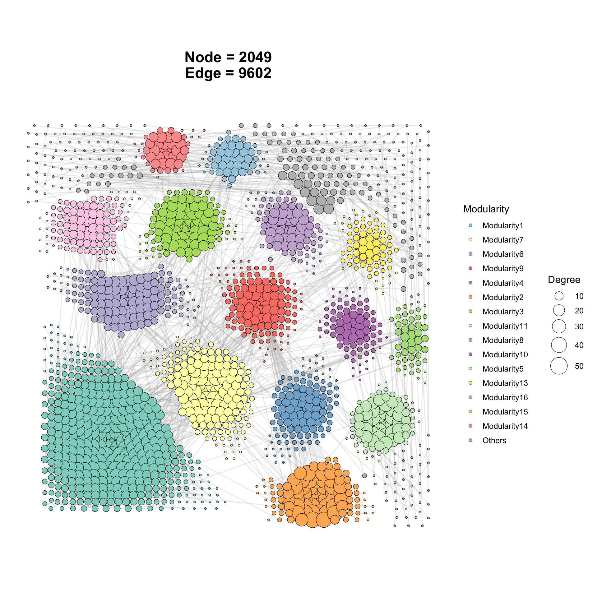
6.1.6 Petal layout
# "petal": each module is laid out as a circular petal radiating from the
# global centre. Visually emphasises modular structure.
p <- ggNetView(
  graph_obj     = graph_obj,
  layout        = "petal",
  center        = F,
  shrink        = 0.8,
  layout.module = "adjacent",
  group.by      = "Modularity",
  fill.by       = "Modularity"
)

p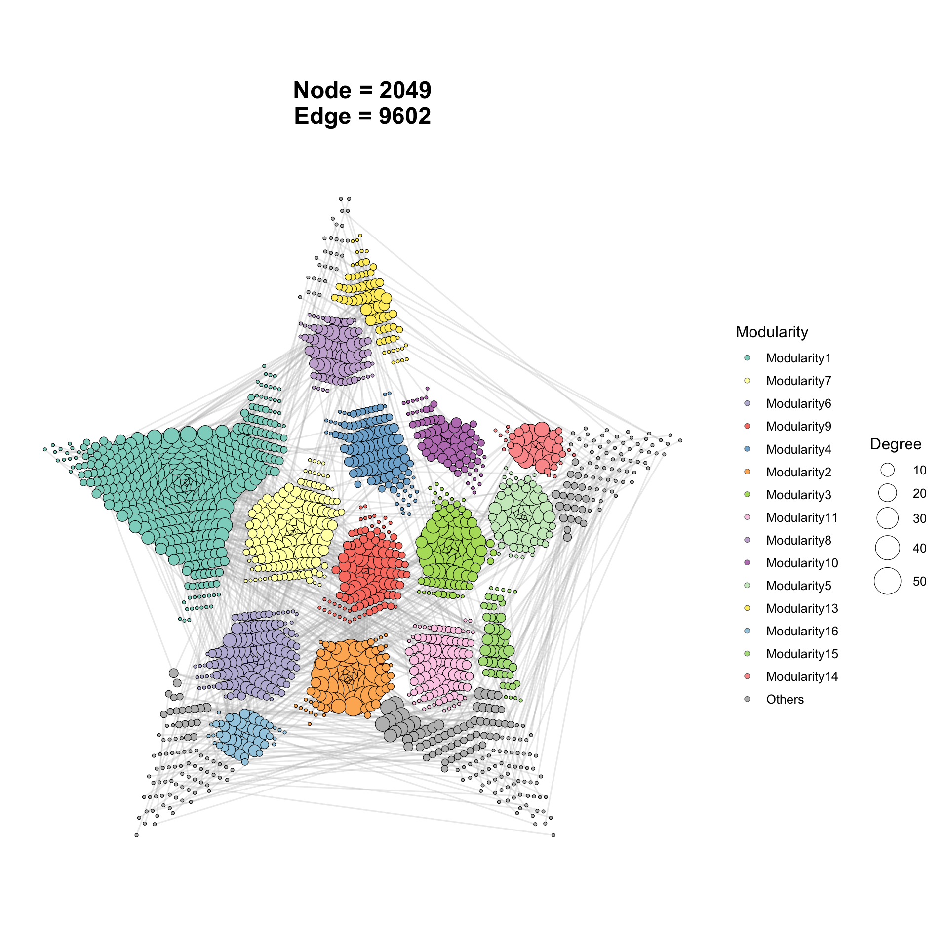
6.1.7 Circle layout
# "circle": all nodes placed on a single ring. Useful for small networks or for
# emphasising edges over node positions.
p <- ggNetView(
  graph_obj     = graph_obj,
  layout        = "circle",
  center        = F,
  shrink        = 0.8,
  layout.module = "adjacent",
  group.by      = "Modularity",
  fill.by       = "Modularity"
)

p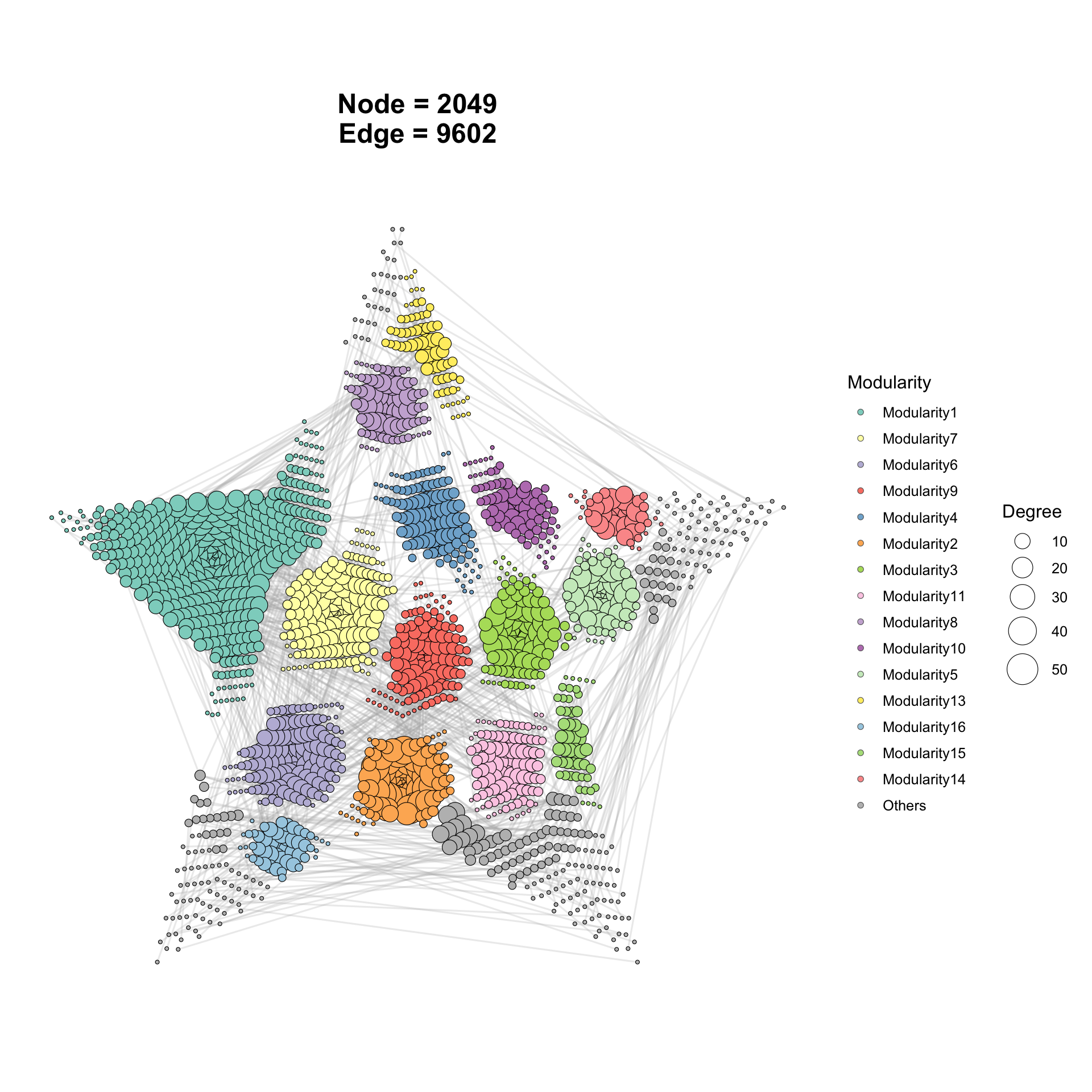
6.1.8 Diamond outline layout
# "diamond_outline": diamond layout but nodes pushed toward the module border —
# hollow-looking modules, easier to read edge connections inside each module.
p <- ggNetView(
  graph_obj     = graph_obj,
  layout        = "diamond_outline",
  center        = F,
  shrink        = 0.8,
  layout.module = "adjacent",
  group.by      = "Modularity",
  fill.by       = "Modularity"
)

p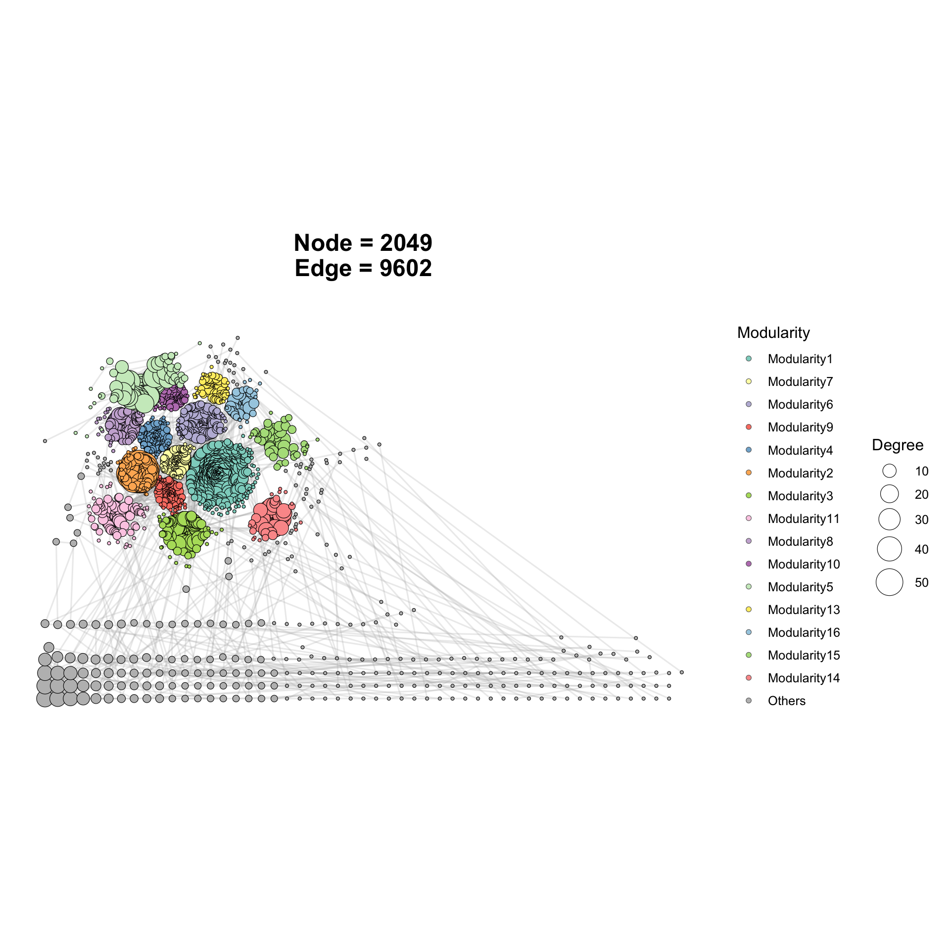
6.1.9 Grid layout
# "grid": nodes snapped to a regular rectangular grid.
# Edges may cross a lot, but useful for systematic comparison plots.
p <- ggNetView(
  graph_obj     = graph_obj,
  layout        = "grid",
  center        = F,
  shrink        = 0.8,
  layout.module = "adjacent",
  group.by      = "Modularity",
  fill.by       = "Modularity"
)

p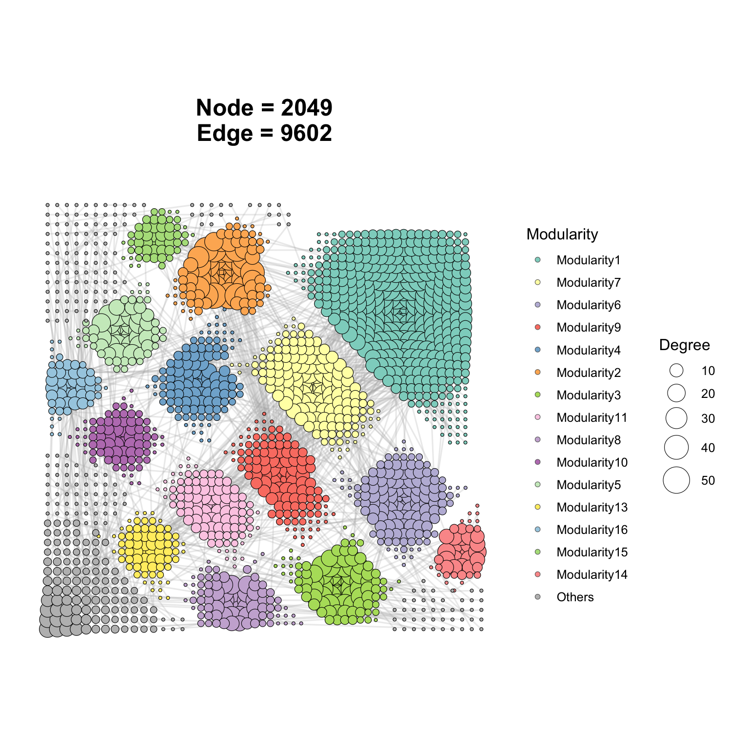
6.1.10 Heart_centered layout
# "heart_centered": stylised heart-shaped frame with nodes pulled toward the
# centre. Mostly cosmetic — handy for talks / decorative figures.
p <- ggNetView(
  graph_obj     = graph_obj,
  layout        = "heart_centered",
  center        = F,
  shrink        = 0.8,
  layout.module = "adjacent",
  group.by      = "Modularity",
  fill.by       = "Modularity"
)

p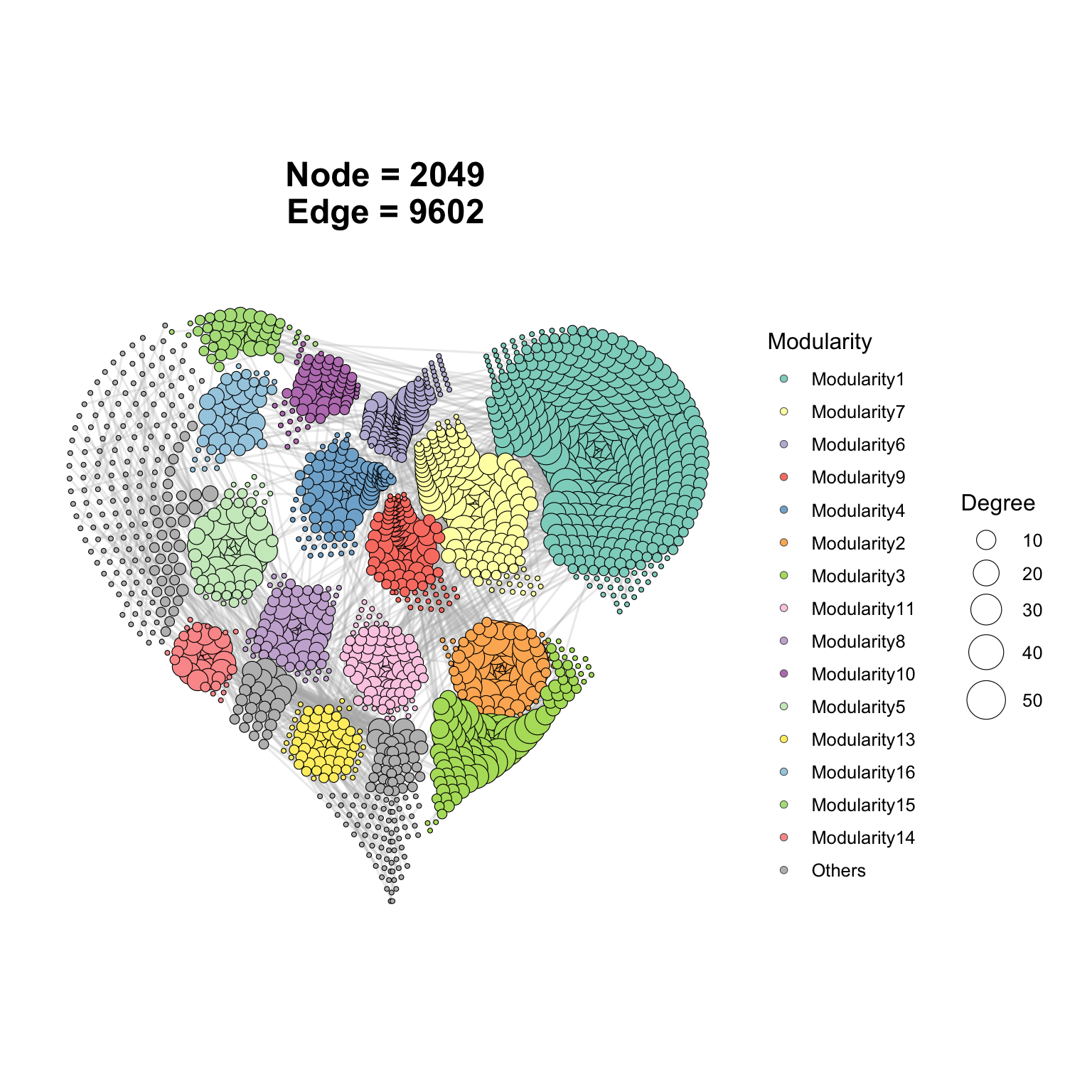
6.1.11 Lgl layout
# "lgl" (Large Graph Layout): force-directed layout designed for large graphs;
# spreads nodes radially around dense cores. Scales better than FR/KK.
p <- ggNetView(
  graph_obj     = graph_obj,
  layout        = "lgl",
  center        = F,
  shrink        = 0.8,
  layout.module = "adjacent",
  group.by      = "Modularity",
  fill.by       = "Modularity"
)
## Warning in alg_fun(graph): LGL layout does not support disconnected graphs yet.
## Source: layout/large_graph.c:179## Warning in ggNetView(graph_obj = graph_obj, layout = "lgl", center = F, :
## `layout.module = 'adjacent'` failed at k_nn = 12; retrying with k_nn = 32.
p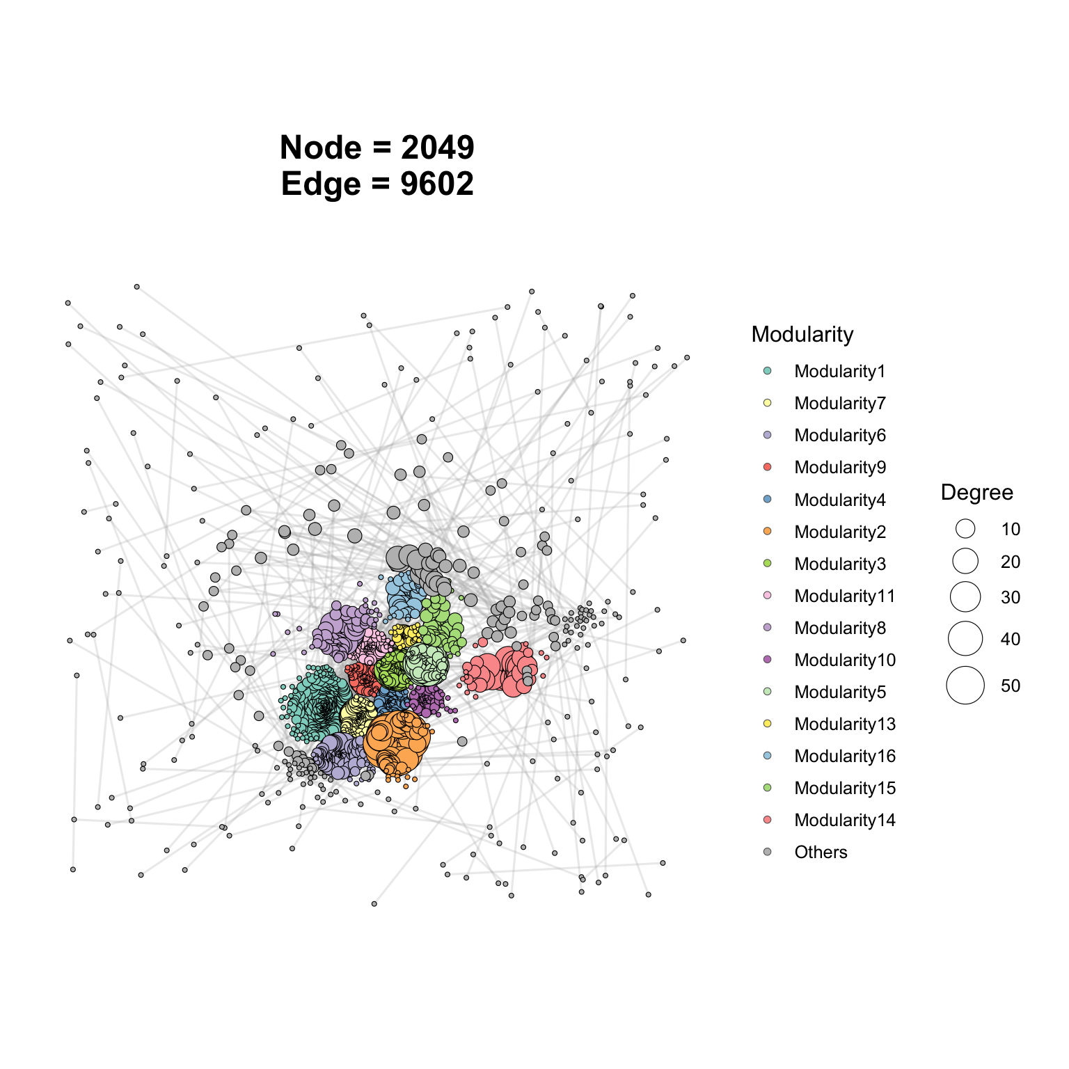
6.1.12 Randomly layout
# "randomly": nodes placed at uniformly random positions inside the canvas.
# Baseline / sanity-check layout — not informative on its own.
p <- ggNetView(
  graph_obj     = graph_obj,
  layout        = "randomly",
  center        = F,
  shrink        = 0.8,
  layout.module = "adjacent",
  group.by      = "Modularity",
  fill.by       = "Modularity"
)

p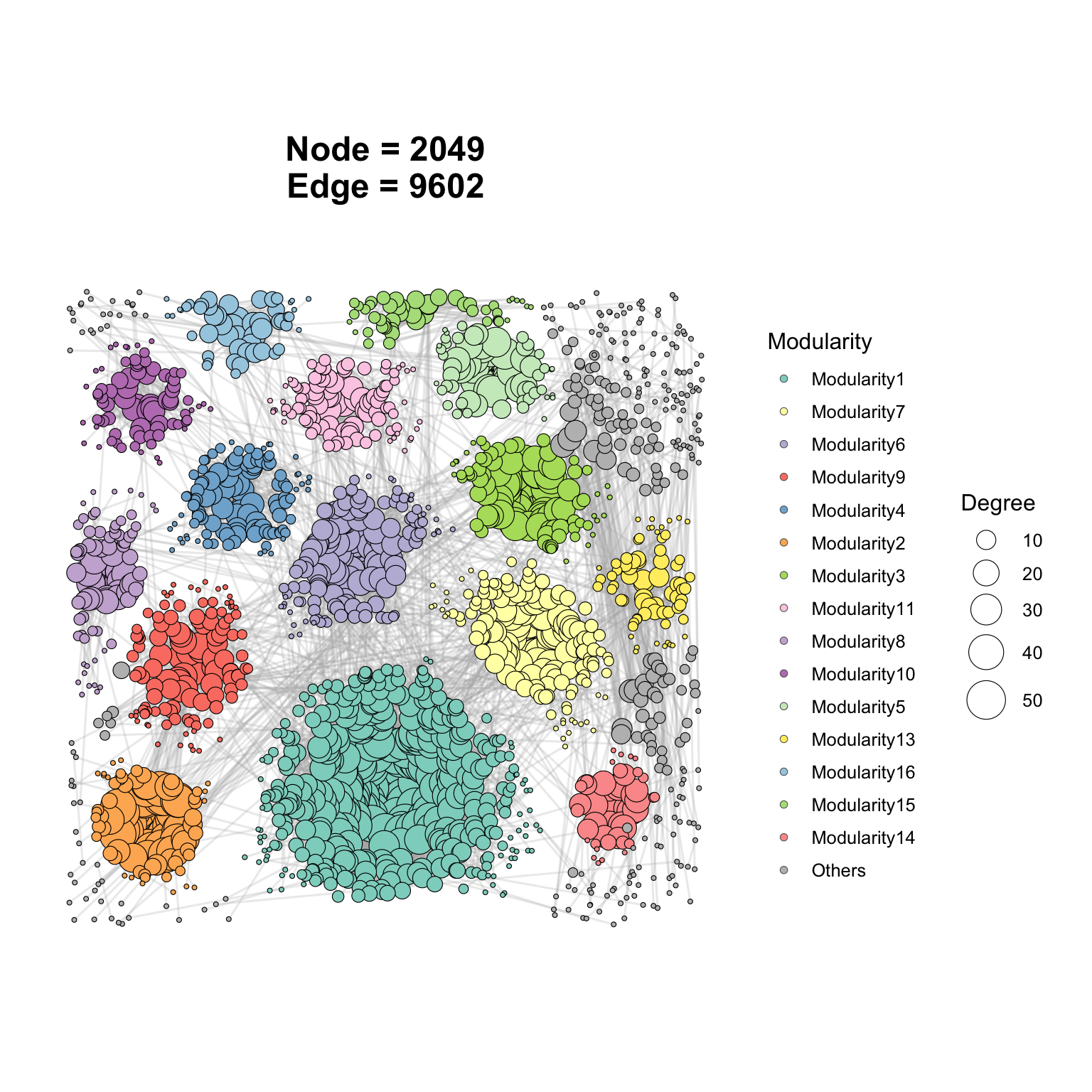
6.1.13 Rectangle layout
# "rectangle": nodes laid out along a rectangular frame.
# Good when you want to free up the centre for annotations / edge bundles.
p <- ggNetView(
  graph_obj     = graph_obj,
  layout        = "rectangle",
  center        = F,
  shrink        = 0.8,
  layout.module = "adjacent",
  group.by      = "Modularity",
  fill.by       = "Modularity"
)

p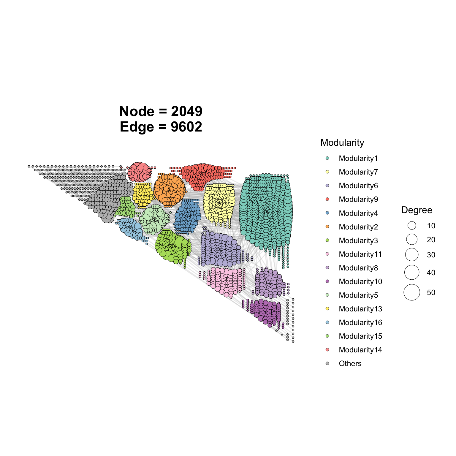
6.1.14 Square layout
# "square": like rectangle but constrained to a square aspect ratio.
p <- ggNetView(
  graph_obj     = graph_obj,
  layout        = "square",
  center        = F,
  shrink        = 0.8,
  layout.module = "adjacent",
  group.by      = "Modularity",
  fill.by       = "Modularity"
)

p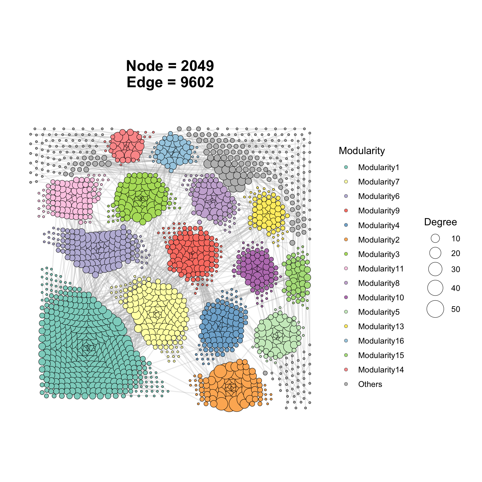
6.1.15 Star layout
# "star": one central node + others arranged as rays radiating outward.
# Best when there is a clear hub node; less useful for community-rich graphs.
p <- ggNetView(
  graph_obj     = graph_obj,
  layout        = "star",
  center        = F,
  shrink        = 0.8,
  layout.module = "adjacent",
  group.by      = "Modularity",
  fill.by       = "Modularity"
)

p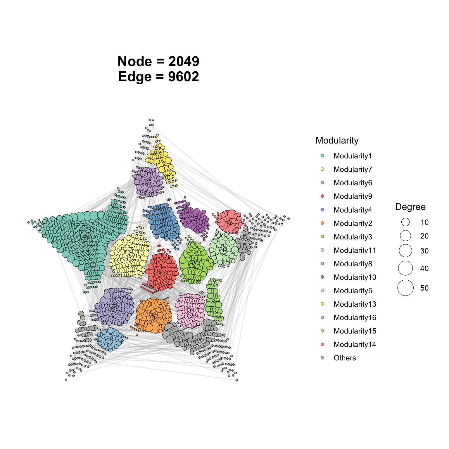
6.1.16 Star_concentric layout
# "star_concentric": star layout with multiple concentric rings — nodes ranked
# by some centrality measure end up closer to the centre.
p <- ggNetView(
  graph_obj     = graph_obj,
  layout        = "star_concentric",
  center        = F,
  shrink        = 0.8,
  layout.module = "adjacent",
  group.by      = "Modularity",
  fill.by       = "Modularity"
)

p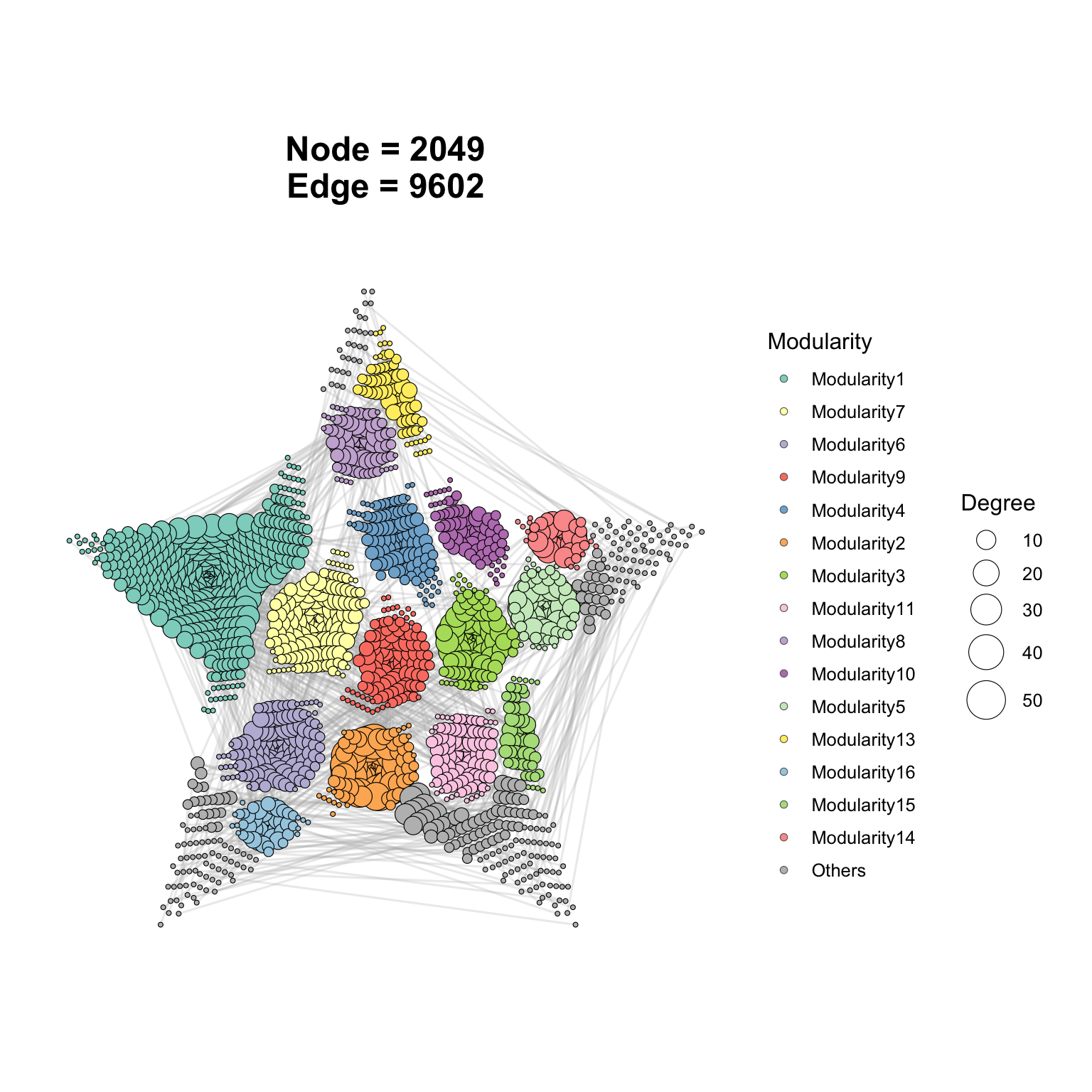
6.1.17 Stress layout
# "stress": stress-majorisation layout (from graphlayouts). Generally produces
# the cleanest "FR/KK-like" results and is reproducible across runs — a strong
# default for publication figures.
p <- ggNetView(
  graph_obj     = graph_obj,
  layout        = "stress",
  center        = F,
  shrink        = 0.8,
  layout.module = "adjacent",
  group.by      = "Modularity",
  fill.by       = "Modularity"
)
## Warning in ggNetView(graph_obj = graph_obj, layout = "stress", center = F, :
## `layout.module = 'adjacent'` failed at k_nn = 12; retrying with k_nn = 32.
p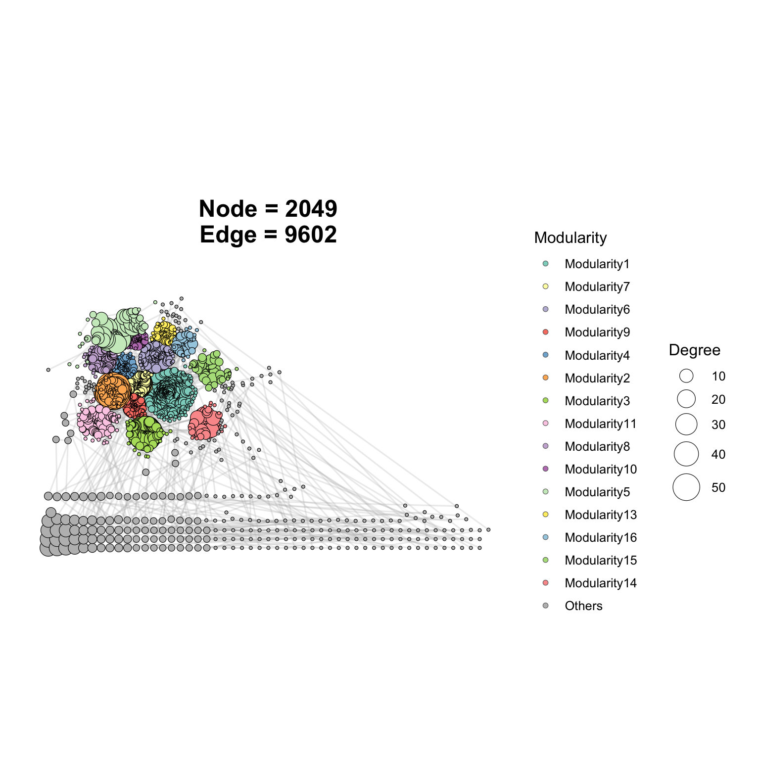
6.1.18 circular_modules_gephi_layout
p_modules_gephi <- ggNetView(
  graph_obj = graph_obj,
  layout = "circular_modules_gephi_layout",
  center = F,
  shrink = 0.9,
  pointsize = c(1, 5),
  layout.module = "order",
  group.by = "Modularity",
  fill.by = "Modularity",
  anchor_dist = 60,
  mapping_line = T,
  r = 1
)

p_modules_gephi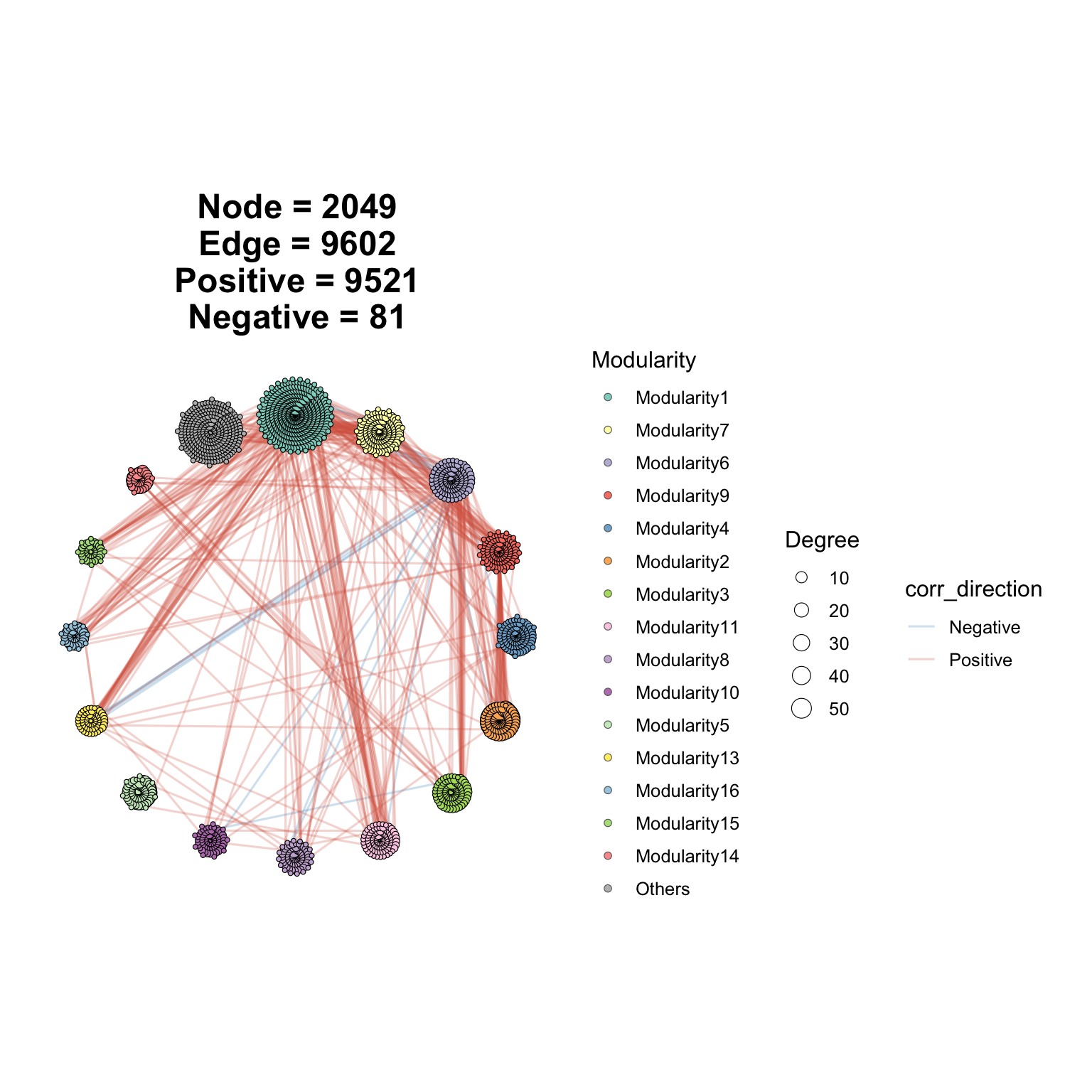
p_modules_equal_gephi <- ggNetView(
  graph_obj = graph_obj,
  layout = "circular_modules_equal_gephi_layout",
  center = F,
  shrink = 0.9,
  pointsize = c(1, 5),
  layout.module = "order",
  group.by = "Modularity",
  fill.by = "Modularity",
  anchor_dist = 60,
  mapping_line = T,
  r = 1
)

p_modules_equal_gephi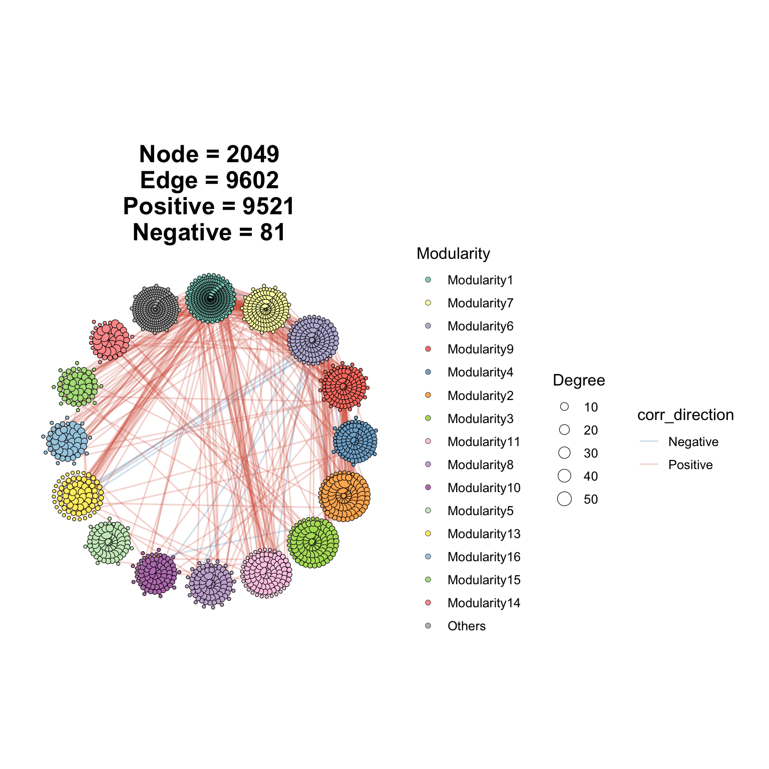
6.1.19 consensus_module_gephi
p_consensus_module <- ggNetView(
  graph_obj = graph_obj,
  layout = "consensus_module_gephi",
  center = F,
  r = 2,
  node_add = 7,
  anchor_dist = 50,
  pointsize = c(1,3),
  layout.module = "order"
)

p_consensus_module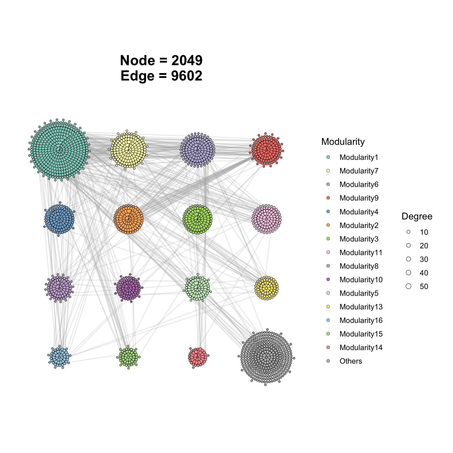
p_consensus_module2 <- ggNetView(
  graph_obj = graph_obj,
  layout = "consensus_module_gephi",
  center = F,
  r = 2,
  node_add = 7,
  anchor_dist = 50,
  pointsize = c(1,3),
  add_outer = T,
  expand_outer = 1.3,
  label = T,
  layout.module = "order"
)
## Coordinate system already present.
## ℹ Adding new coordinate system, which will replace the existing one.
p_consensus_module2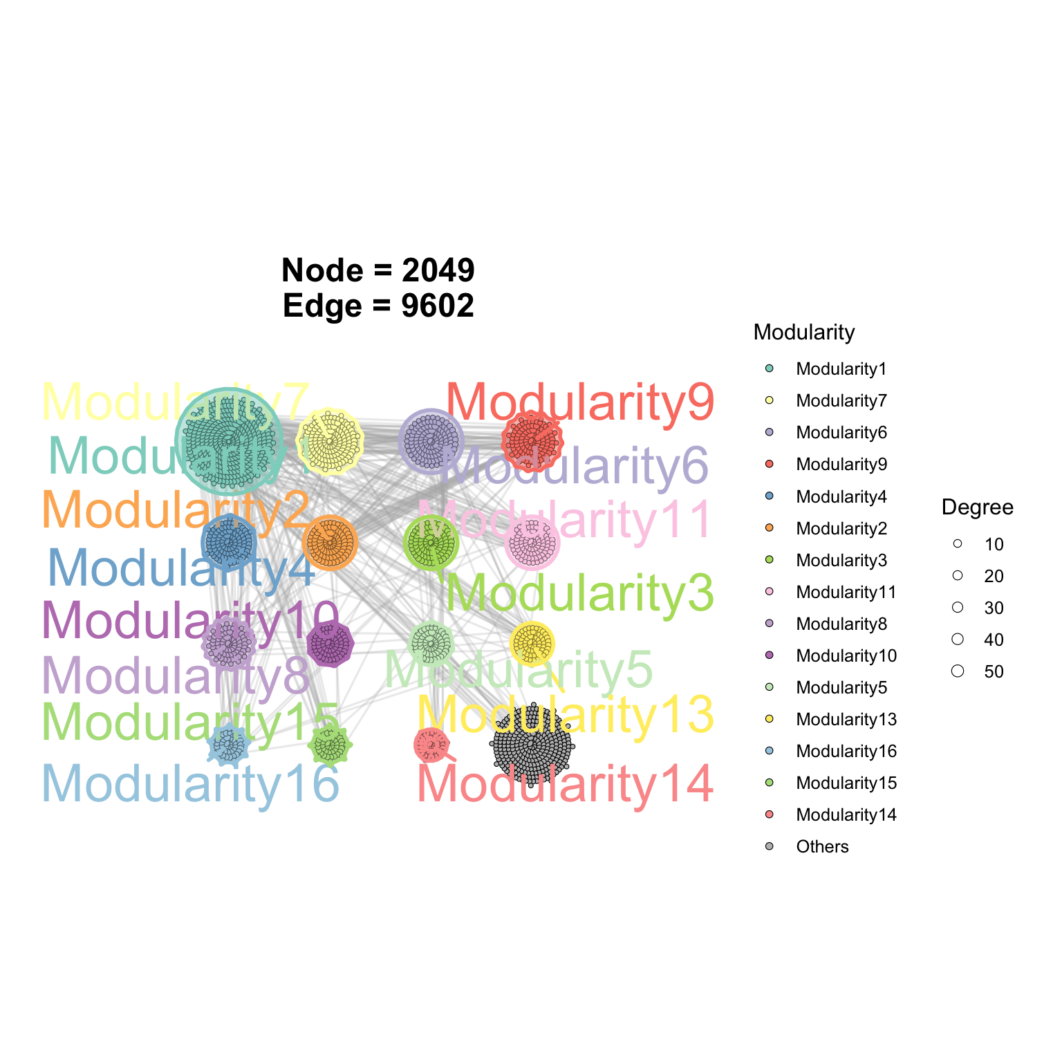
6.1.20 consensus_module_equal_gephi
p_consensus_module3 <- ggNetView(
  graph_obj = graph_obj,
  layout = "consensus_module_equal_gephi",
  center = F,
  r = 2,
  node_add = 7,
  anchor_dist = 50,
  pointsize = c(1,3),
  layout.module = "order"
)

p_consensus_module3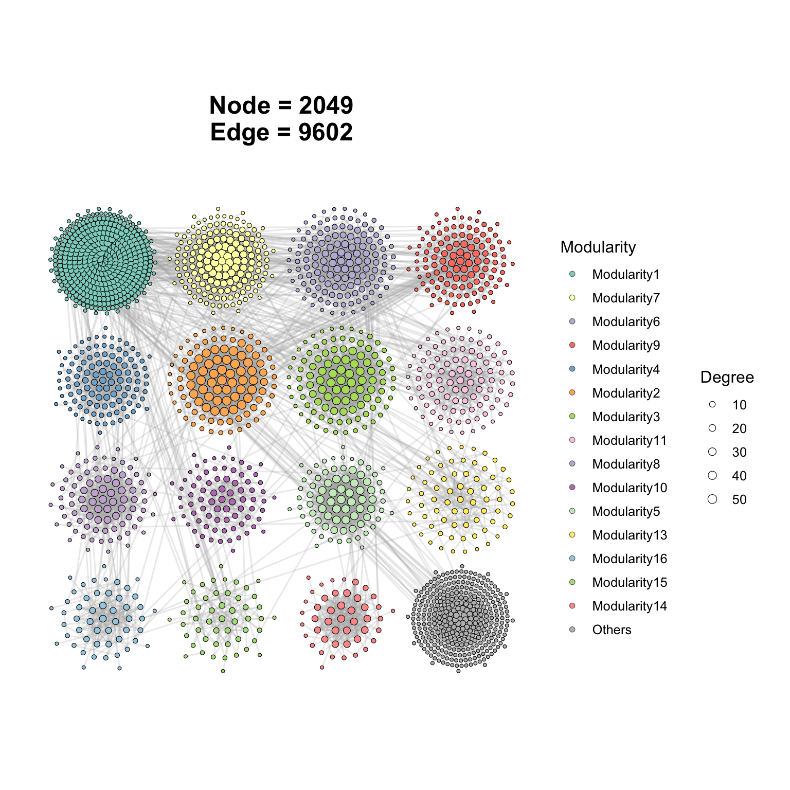
p_consensus_module4 <- ggNetView(
  graph_obj = graph_obj,
  layout = "consensus_module_equal_gephi",
  fill.by = "Phylum",
  center = F,
  r = 2,
  node_add = 7,
  anchor_dist = 50,
  pointsize = c(1,3),
  layout.module = "order"
)

p_consensus_module4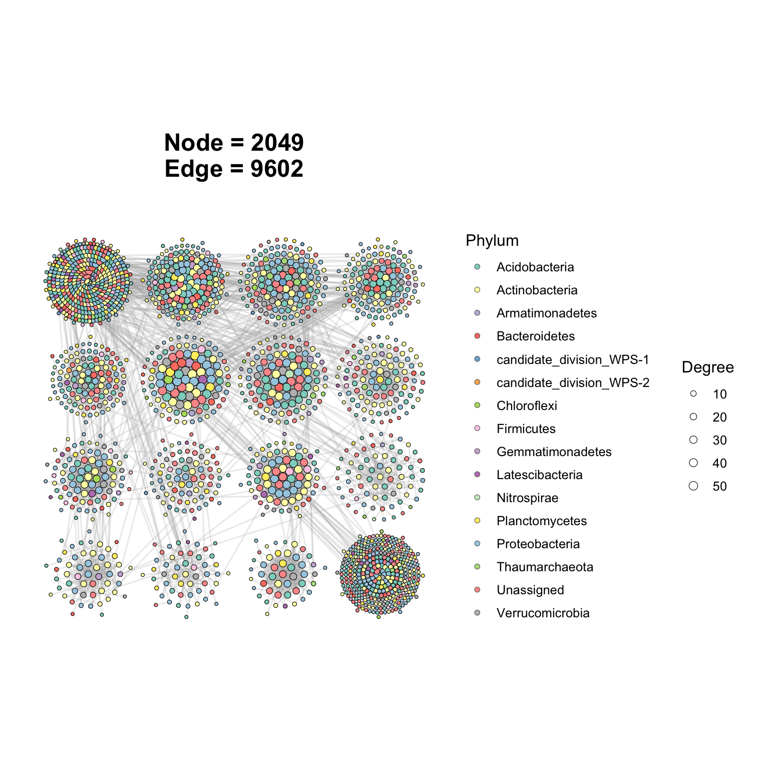
p_consensus_module5 <- ggNetView(
  graph_obj = graph_obj,
  layout = "consensus_module_equal_gephi",
  fill.by = "Phylum",
  center = F,
  r = 2,
  node_add = 7,
  anchor_dist = 50,
  pointsize = c(1,3),
  add_outer = T,
  expand_outer = 1.3,
  label = T,
  layout.module = "order"
)
## Coordinate system already present.
## ℹ Adding new coordinate system, which will replace the existing one.
p_consensus_module5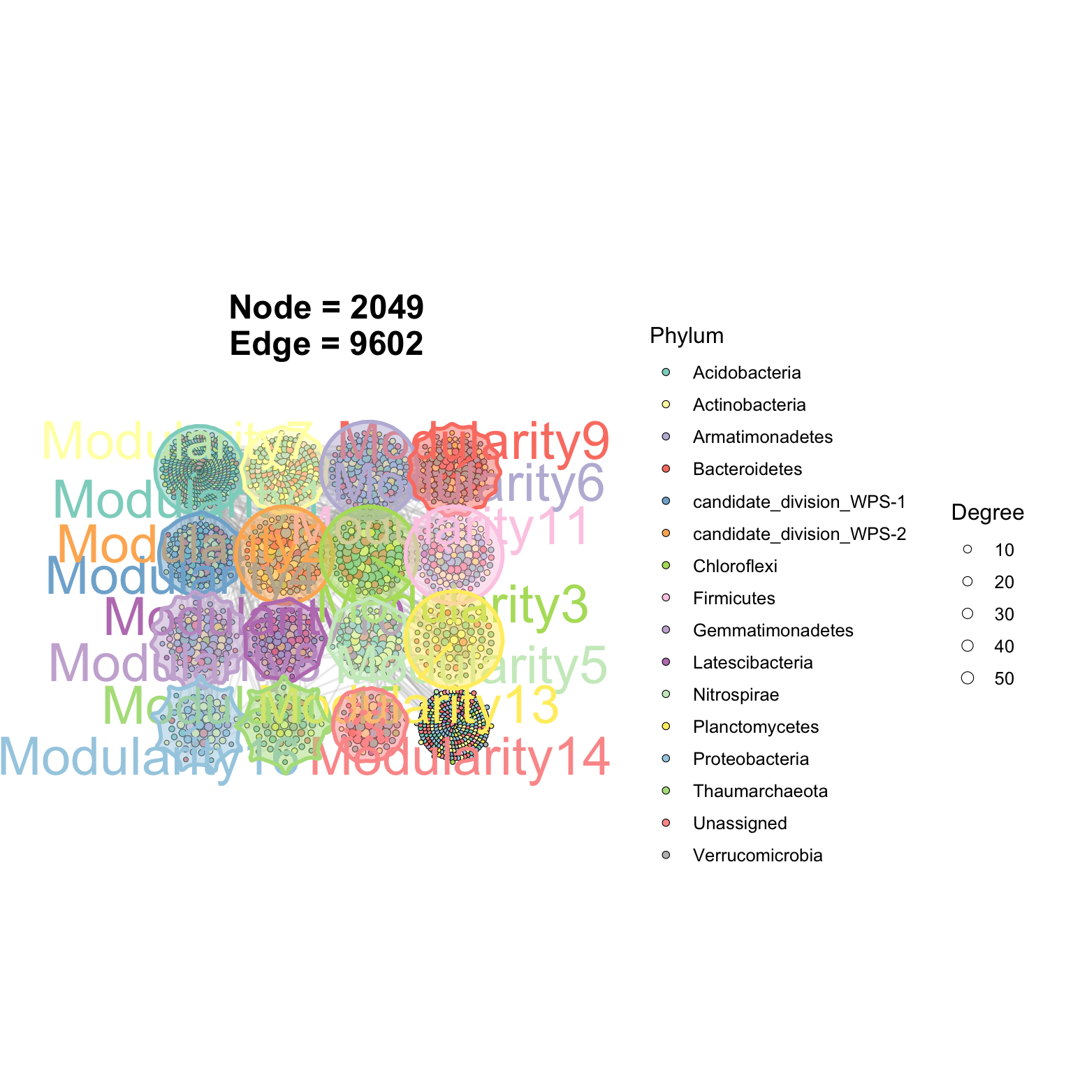
6.2 Sub graph layout
6.2.1 bipartite network
# Extract the subgraph corresponding to module "1" and "7".
# Internally, get_subgraph():
#   1) splits all nodes by the `Modularity` attribute,
#   2) builds one subgraph per module and stores them in `sub_graph_all`,
#   3) if `select_module` is provided, also returns `sub_graph_select`
#      (the graph filtered to those modules via tidygraph::filter),
#   4) returns `stat_module`: a table of node counts per module across the full graph.
graph_sub <- get_subgraph(graph_obj = graph_obj,
                          select_module = c("1", "7")
                          )
## Module Number
## 1 1 416
## 2 7 161
## 3 6 137
## 4 9 121
## 5 4 112
## 6 2 105
## 7 3 104
## 8 11 101
## 9 8 87
## 10 10 80
## 11 5 78
## 12 13 70
## 13 16 52
## 14 15 51
## 15 14 46
## 16 Others 328
graph_sub$sub_graph_select## # A tbl_graph: 577 nodes and 3865 edges
## #
## # An undirected simple graph with 1 component
## #
## # Node Data: 577 × 14 (active)
## name modularity modularity2 modularity3 Modularity Degree Strength Kingdom
## <chr> <fct> <ord> <chr> <ord> <dbl> <dbl> <chr>
## 1 ASV_916 1 1 1 1 58 50.5 Bacter…
## 2 ASV_777 1 1 1 1 58 48.7 Bacter…
## 3 ASV_606 1 1 1 1 55 45.8 Bacter…
## 4 ASV_740 1 1 1 1 54 47.2 Bacter…
## 5 ASV_14… 1 1 1 1 54 44.5 Bacter…
## 6 ASV_23… 1 1 1 1 54 47.4 Bacter…
## 7 ASV_15… 1 1 1 1 52 45.3 Bacter…
## 8 ASV_24… 1 1 1 1 52 43.0 Bacter…
## 9 ASV_19… 1 1 1 1 52 43.0 Bacter…
## 10 ASV_568 1 1 1 1 51 45.1 Bacter…
## # ℹ 567 more rows
## # ℹ 6 more variables: Phylum <chr>, Class <chr>, Order <chr>, Family <chr>,
## # Genus <chr>, Species <chr>
## #
## # Edge Data: 3,865 × 5
## from to weight correlation corr_direction
## <int> <int> <dbl> <dbl> <chr>
## 1 197 337 0.798 -0.798 Negative
## 2 210 337 0.801 -0.801 Negative
## 3 35 196 0.828 0.828 Positive
## # ℹ 3,862 more rows6.2.1.1 bipartite_layout
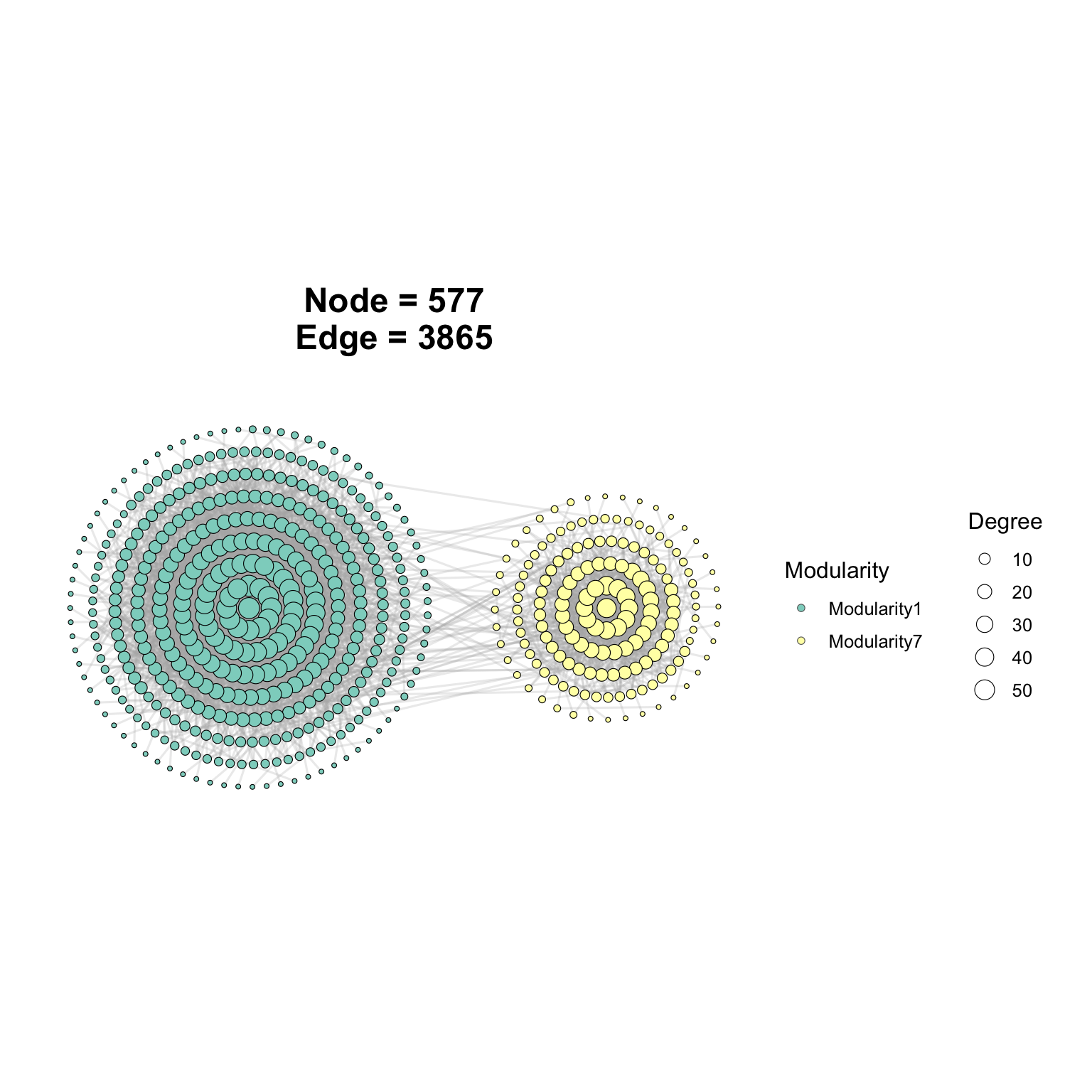
p1 <- ggNetView(
  graph_obj = graph_sub$sub_graph_select,
  layout = "bipartite_layout",
  layout.module = "order",
  center = F,
  scale = T
)

p1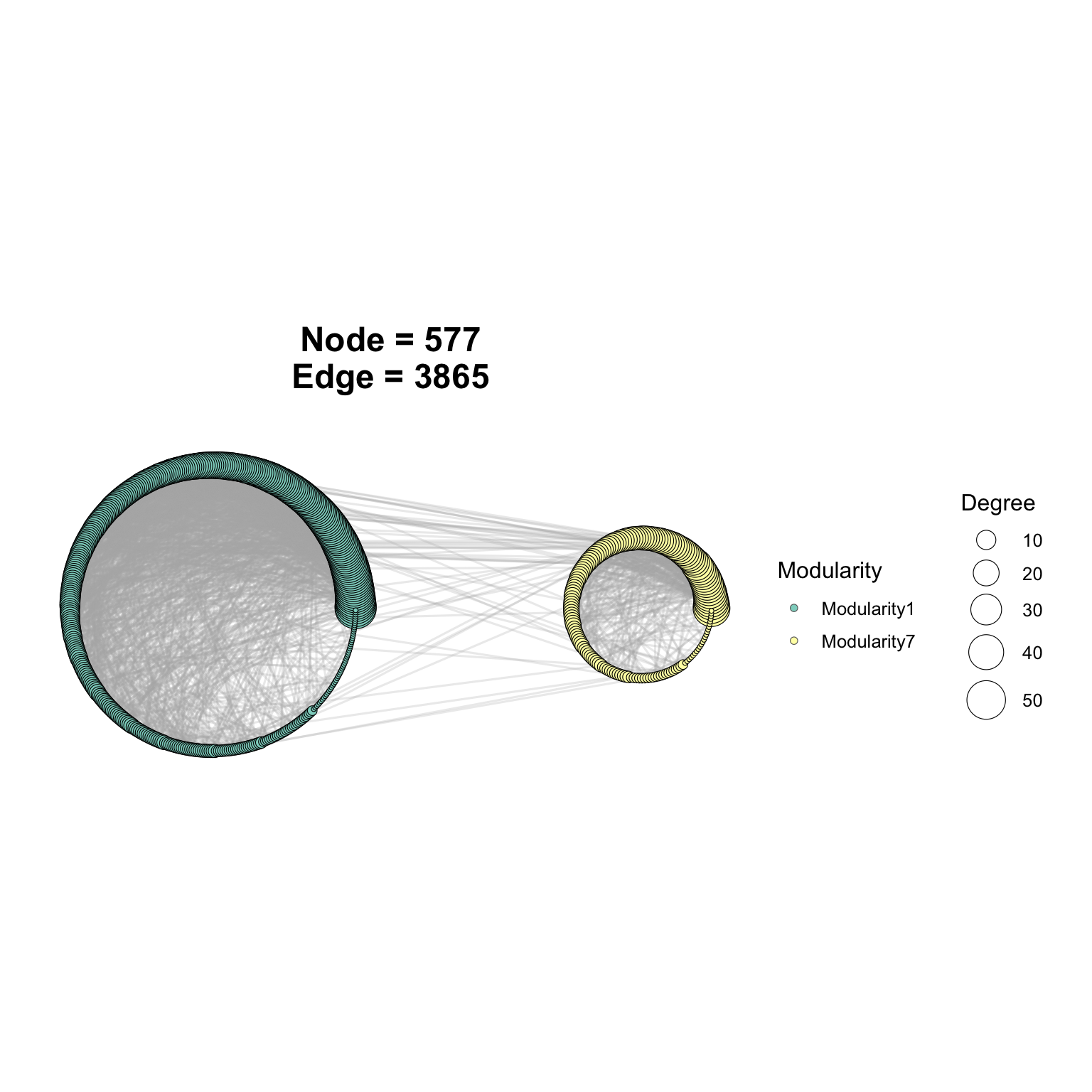
6.2.2 tripartite network
graph_sub <- get_subgraph(graph_obj = graph_obj,
                          select_module = c("1", "7", "6")
                          )
## Module Number
## 1 1 416
## 2 7 161
## 3 6 137
## 4 9 121
## 5 4 112
## 6 2 105
## 7 3 104
## 8 11 101
## 9 8 87
## 10 10 80
## 11 5 78
## 12 13 70
## 13 16 52
## 14 15 51
## 15 14 46
## 16 Others 328
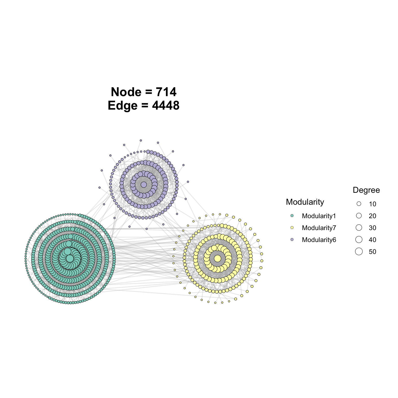
graph_sub$sub_graph_select## # A tbl_graph: 714 nodes and 4448 edges
## #
## # An undirected simple graph with 1 component
## #
## # Node Data: 714 × 14 (active)
## name modularity modularity2 modularity3 Modularity Degree Strength Kingdom
## <chr> <fct> <ord> <chr> <ord> <dbl> <dbl> <chr>
## 1 ASV_916 1 1 1 1 58 50.5 Bacter…
## 2 ASV_777 1 1 1 1 58 48.7 Bacter…
## 3 ASV_606 1 1 1 1 55 45.8 Bacter…
## 4 ASV_740 1 1 1 1 54 47.2 Bacter…
## 5 ASV_14… 1 1 1 1 54 44.5 Bacter…
## 6 ASV_23… 1 1 1 1 54 47.4 Bacter…
## 7 ASV_15… 1 1 1 1 52 45.3 Bacter…
## 8 ASV_24… 1 1 1 1 52 43.0 Bacter…
## 9 ASV_19… 1 1 1 1 52 43.0 Bacter…
## 10 ASV_568 1 1 1 1 51 45.1 Bacter…
## # ℹ 704 more rows
## # ℹ 6 more variables: Phylum <chr>, Class <chr>, Order <chr>, Family <chr>,
## # Genus <chr>, Species <chr>
## #
## # Edge Data: 4,448 × 5
## from to weight correlation corr_direction
## <int> <int> <dbl> <dbl> <chr>
## 1 594 597 0.895 0.895 Positive
## 2 588 597 0.864 0.864 Positive
## 3 589 597 0.800 0.800 Positive
## # ℹ 4,445 more rows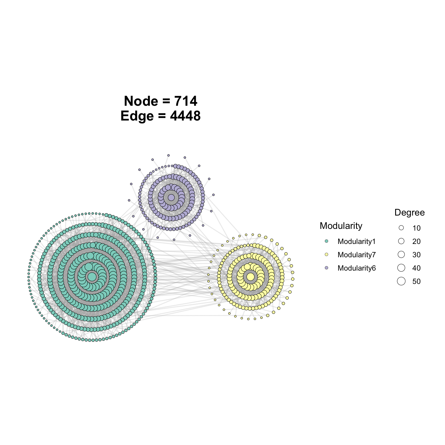
6.2.3 quadripartite network
graph_sub <- get_subgraph(graph_obj = graph_obj,
                          select_module = c("1", "7", "6", "9")
                          )
## Module Number
## 1 1 416
## 2 7 161
## 3 6 137
## 4 9 121
## 5 4 112
## 6 2 105
## 7 3 104
## 8 11 101
## 9 8 87
## 10 10 80
## 11 5 78
## 12 13 70
## 13 16 52
## 14 15 51
## 15 14 46
## 16 Others 328
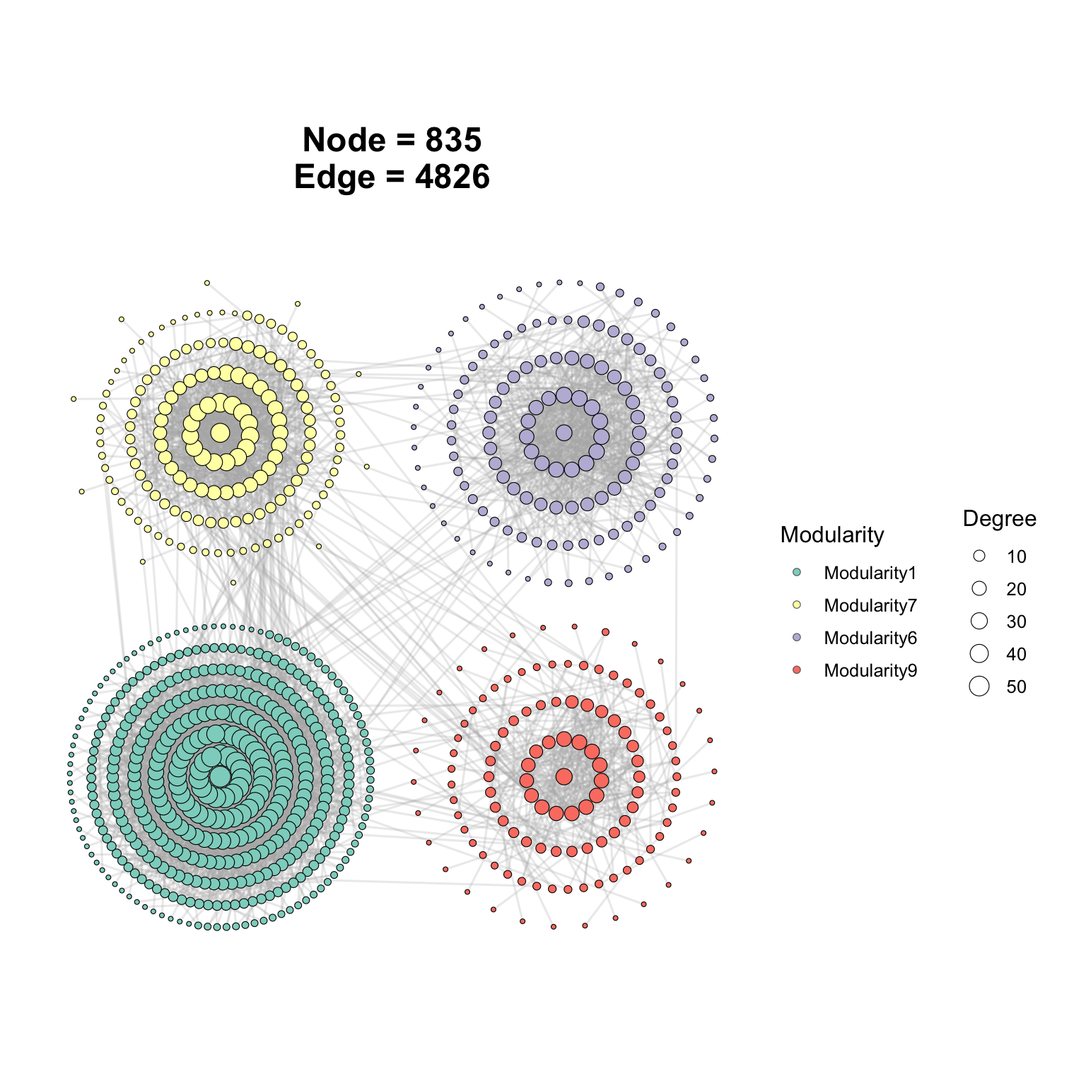
graph_sub$sub_graph_select## # A tbl_graph: 835 nodes and 4826 edges
## #
## # An undirected simple graph with 1 component
## #
## # Node Data: 835 × 14 (active)
## name modularity modularity2 modularity3 Modularity Degree Strength Kingdom
## <chr> <fct> <ord> <chr> <ord> <dbl> <dbl> <chr>
## 1 ASV_916 1 1 1 1 58 50.5 Bacter…
## 2 ASV_777 1 1 1 1 58 48.7 Bacter…
## 3 ASV_606 1 1 1 1 55 45.8 Bacter…
## 4 ASV_740 1 1 1 1 54 47.2 Bacter…
## 5 ASV_14… 1 1 1 1 54 44.5 Bacter…
## 6 ASV_23… 1 1 1 1 54 47.4 Bacter…
## 7 ASV_15… 1 1 1 1 52 45.3 Bacter…
## 8 ASV_24… 1 1 1 1 52 43.0 Bacter…
## 9 ASV_19… 1 1 1 1 52 43.0 Bacter…
## 10 ASV_568 1 1 1 1 51 45.1 Bacter…
## # ℹ 825 more rows
## # ℹ 6 more variables: Phylum <chr>, Class <chr>, Order <chr>, Family <chr>,
## # Genus <chr>, Species <chr>
## #
## # Edge Data: 4,826 × 5
## from to weight correlation corr_direction
## <int> <int> <dbl> <dbl> <chr>
## 1 594 597 0.895 0.895 Positive
## 2 588 597 0.864 0.864 Positive
## 3 589 597 0.800 0.800 Positive
## # ℹ 4,823 more rows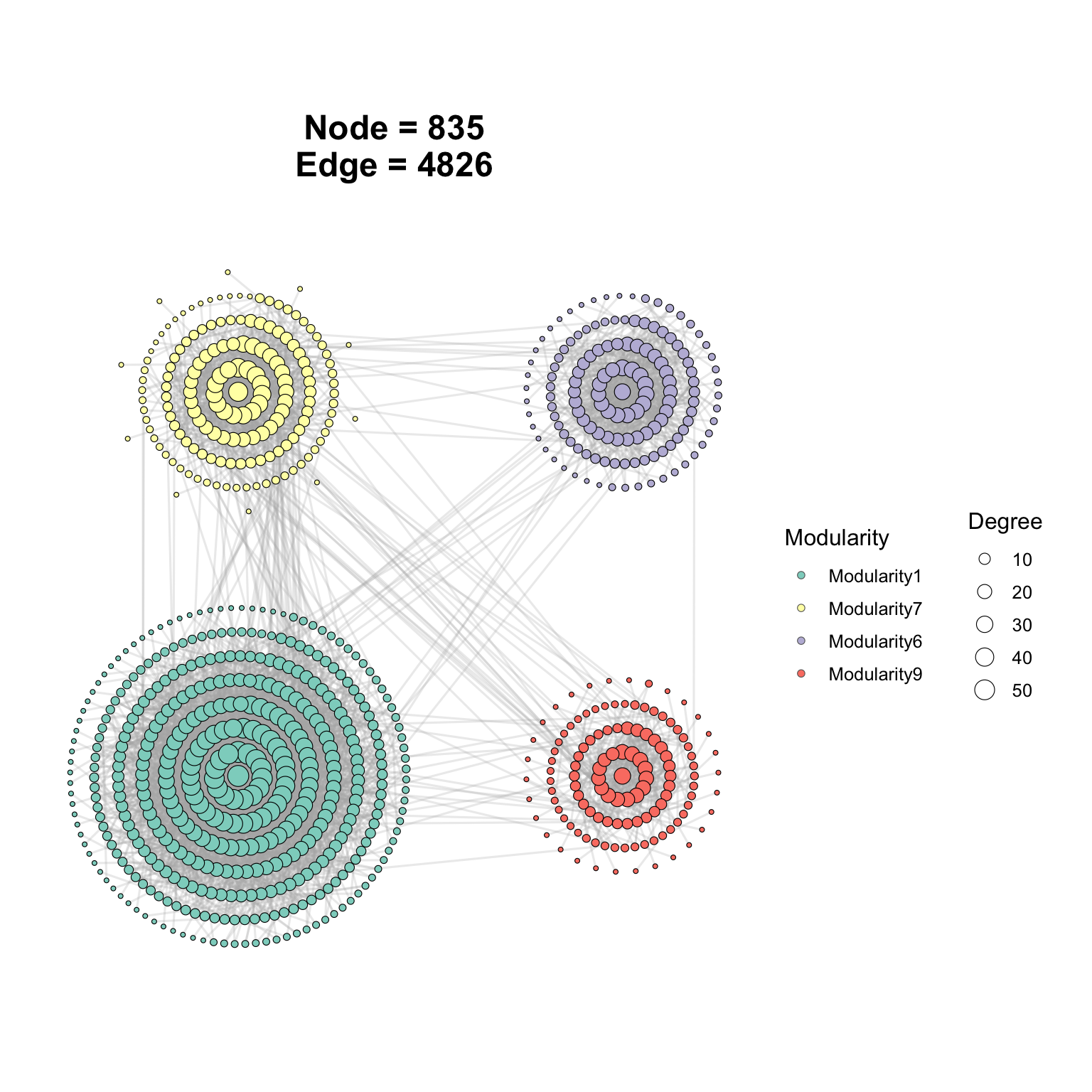
6.2.4 pentapartite network
graph_sub <- get_subgraph(graph_obj = graph_obj,
                          select_module = c("1", "7", "6", "9", "4")
                          )
## Module Number
## 1 1 416
## 2 7 161
## 3 6 137
## 4 9 121
## 5 4 112
## 6 2 105
## 7 3 104
## 8 11 101
## 9 8 87
## 10 10 80
## 11 5 78
## 12 13 70
## 13 16 52
## 14 15 51
## 15 14 46
## 16 Others 328
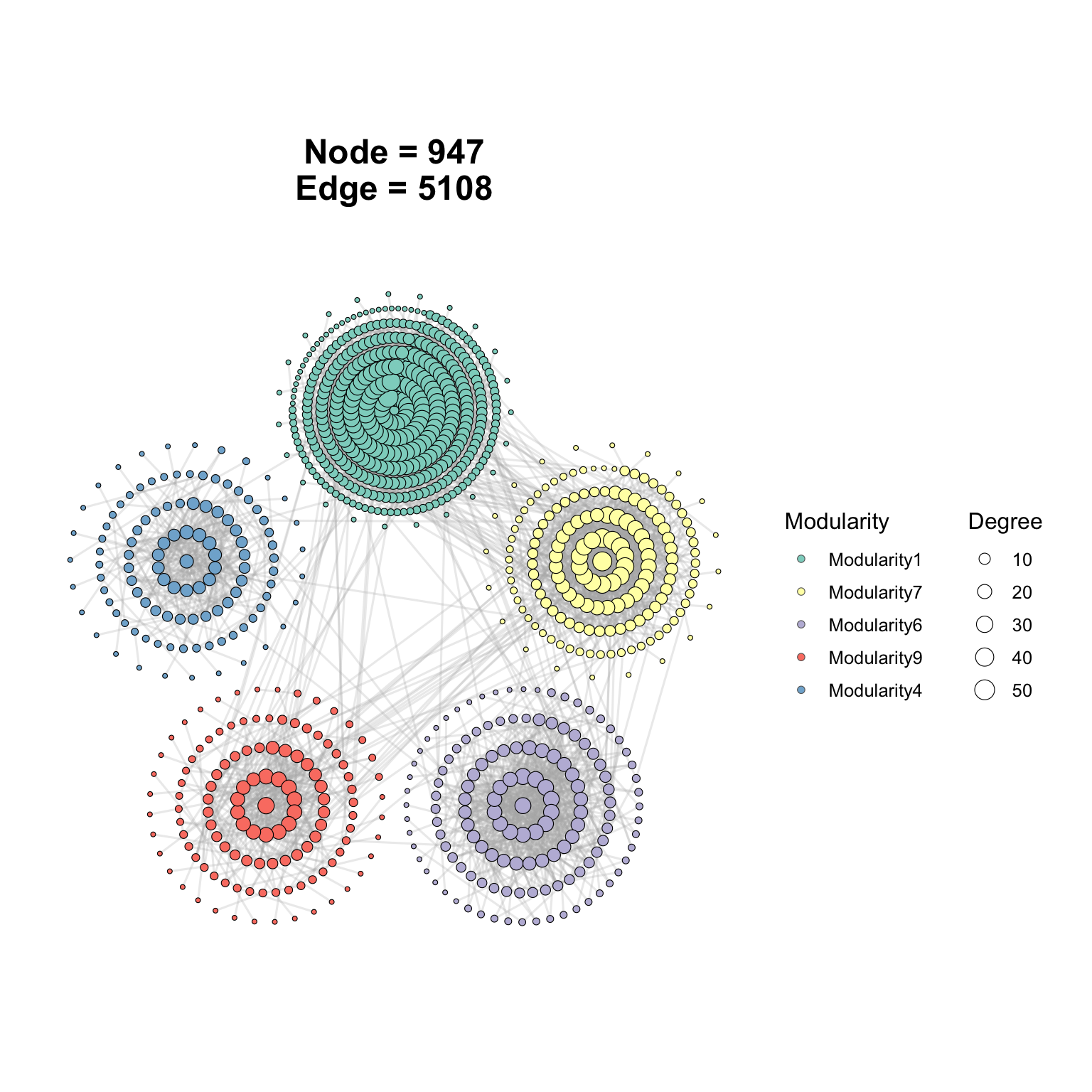
graph_sub$sub_graph_select## # A tbl_graph: 947 nodes and 5108 edges
## #
## # An undirected simple graph with 1 component
## #
## # Node Data: 947 × 14 (active)
## name modularity modularity2 modularity3 Modularity Degree Strength Kingdom
## <chr> <fct> <ord> <chr> <ord> <dbl> <dbl> <chr>
## 1 ASV_916 1 1 1 1 58 50.5 Bacter…
## 2 ASV_777 1 1 1 1 58 48.7 Bacter…
## 3 ASV_606 1 1 1 1 55 45.8 Bacter…
## 4 ASV_740 1 1 1 1 54 47.2 Bacter…
## 5 ASV_14… 1 1 1 1 54 44.5 Bacter…
## 6 ASV_23… 1 1 1 1 54 47.4 Bacter…
## 7 ASV_15… 1 1 1 1 52 45.3 Bacter…
## 8 ASV_24… 1 1 1 1 52 43.0 Bacter…
## 9 ASV_19… 1 1 1 1 52 43.0 Bacter…
## 10 ASV_568 1 1 1 1 51 45.1 Bacter…
## # ℹ 937 more rows
## # ℹ 6 more variables: Phylum <chr>, Class <chr>, Order <chr>, Family <chr>,
## # Genus <chr>, Species <chr>
## #
## # Edge Data: 5,108 × 5
## from to weight correlation corr_direction
## <int> <int> <dbl> <dbl> <chr>
## 1 594 597 0.895 0.895 Positive
## 2 588 597 0.864 0.864 Positive
## 3 589 597 0.800 0.800 Positive
## # ℹ 5,105 more rows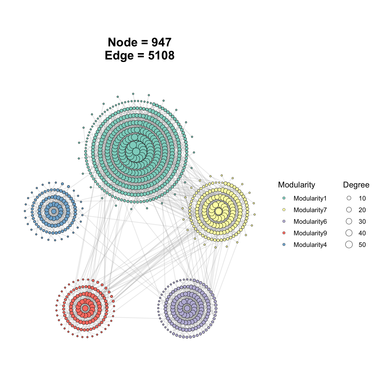
6.2.5 circular network
graph_sub <- get_subgraph(graph_obj = graph_obj,
                          select_module = c("1", "7", "6", "9", "4", "2")
                          )
## Module Number
## 1 1 416
## 2 7 161
## 3 6 137
## 4 9 121
## 5 4 112
## 6 2 105
## 7 3 104
## 8 11 101
## 9 8 87
## 10 10 80
## 11 5 78
## 12 13 70
## 13 16 52
## 14 15 51
## 15 14 46
## 16 Others 328
graph_sub$sub_graph_select## # A tbl_graph: 1052 nodes and 6353 edges
## #
## # An undirected simple graph with 1 component
## #
## # Node Data: 1,052 × 14 (active)
## name modularity modularity2 modularity3 Modularity Degree Strength Kingdom
## <chr> <fct> <ord> <chr> <ord> <dbl> <dbl> <chr>
## 1 ASV_916 1 1 1 1 58 50.5 Bacter…
## 2 ASV_777 1 1 1 1 58 48.7 Bacter…
## 3 ASV_606 1 1 1 1 55 45.8 Bacter…
## 4 ASV_740 1 1 1 1 54 47.2 Bacter…
## 5 ASV_14… 1 1 1 1 54 44.5 Bacter…
## 6 ASV_23… 1 1 1 1 54 47.4 Bacter…
## 7 ASV_15… 1 1 1 1 52 45.3 Bacter…
## 8 ASV_24… 1 1 1 1 52 43.0 Bacter…
## 9 ASV_19… 1 1 1 1 52 43.0 Bacter…
## 10 ASV_568 1 1 1 1 51 45.1 Bacter…
## # ℹ 1,042 more rows
## # ℹ 6 more variables: Phylum <chr>, Class <chr>, Order <chr>, Family <chr>,
## # Genus <chr>, Species <chr>
## #
## # Edge Data: 6,353 × 5
## from to weight correlation corr_direction
## <int> <int> <dbl> <dbl> <chr>
## 1 594 597 0.895 0.895 Positive
## 2 588 597 0.864 0.864 Positive
## 3 589 597 0.800 0.800 Positive
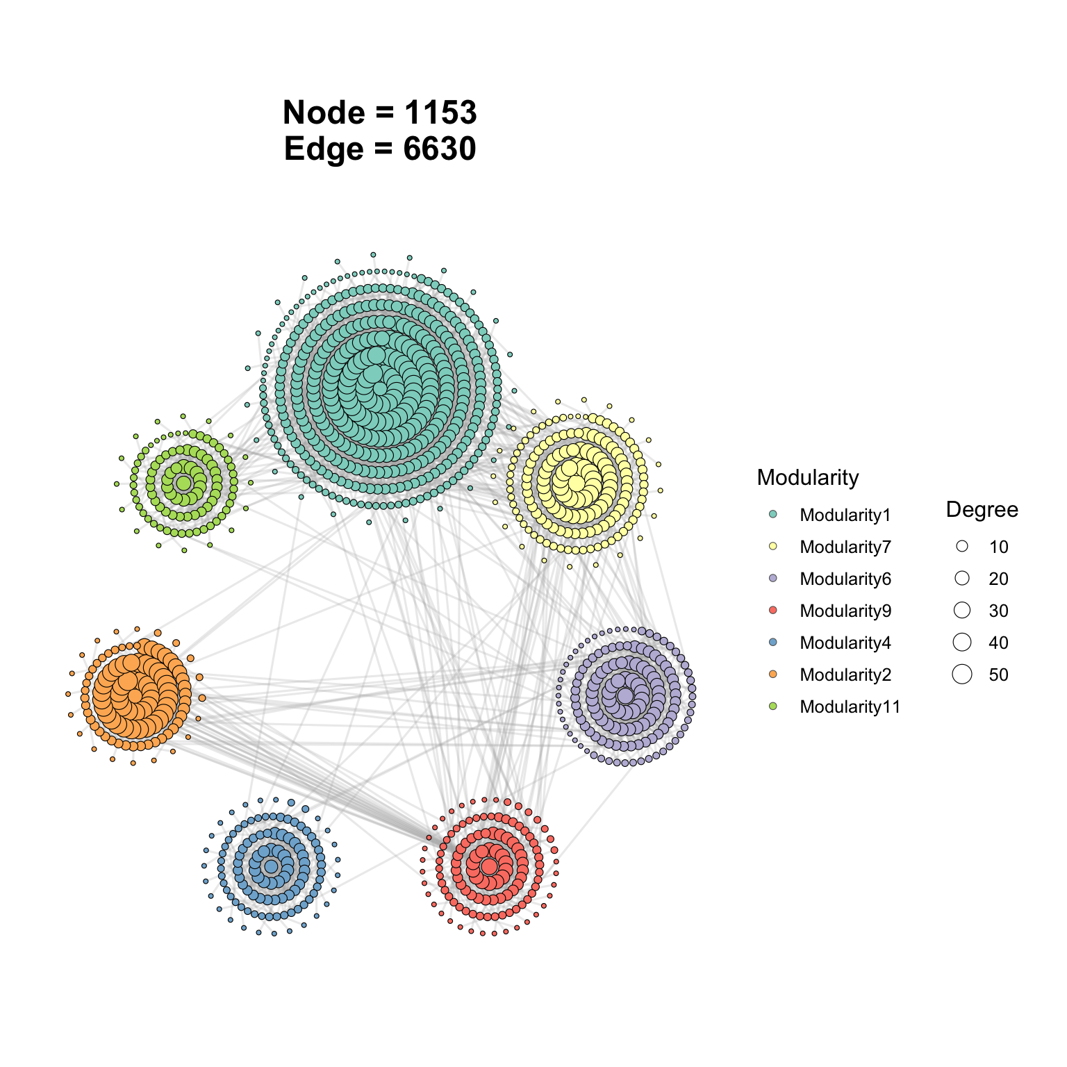
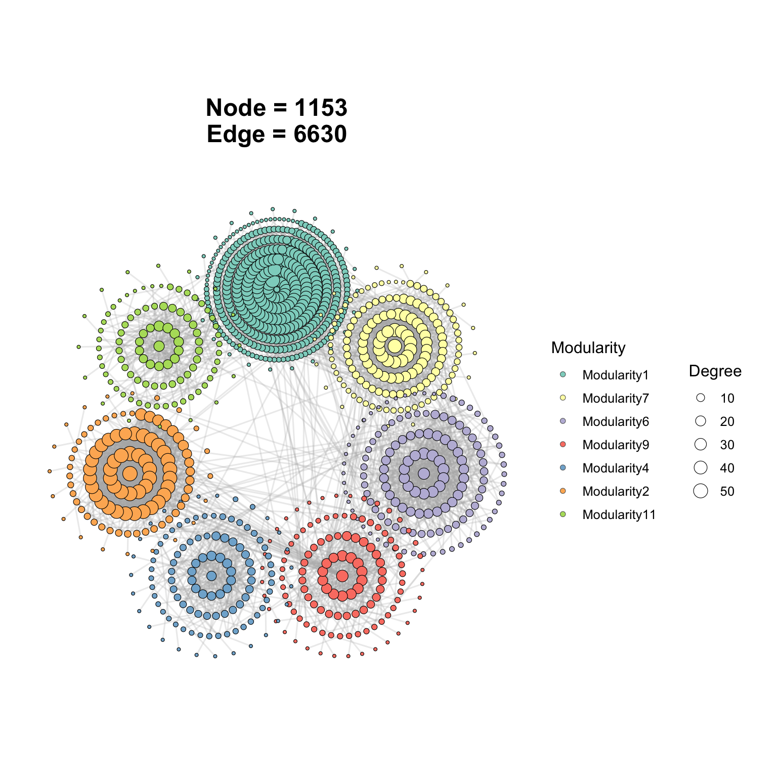
## # ℹ 6,350 more rows6.2.5.1 circular_modules_gephi_layout (six group)
p9 <- ggNetView(
graph_obj = graph_sub$sub_graph_select,
layout = "circular_modules_gephi_layout",
layout.module = "order",
node_add = 14,
anchor_dist = 15,
r = 1,
pointsize = c(1, 5),
mapping_line = F,
center = F,
scale = F
)
p9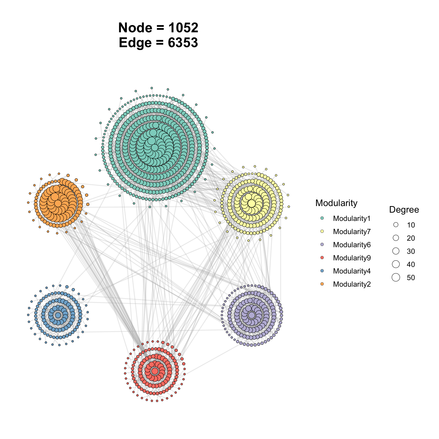 #### circular_modules_equal_gephi_layout (six group)
p10 <- ggNetView(
  graph_obj = graph_sub$sub_graph_select,
  layout = "circular_modules_equal_gephi_layout",
  layout.module = "order",
  node_add = 14,
  anchor_dist = 15,
  r = 1,
  pointsize = c(1, 5),
  mapping_line = F,
  center = F,
  scale = F
)

p10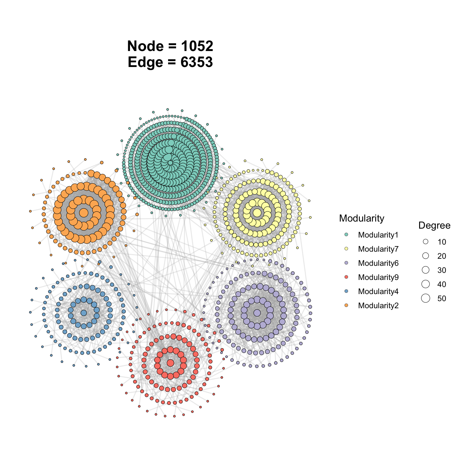
graph_sub <- get_subgraph(graph_obj = graph_obj,
                          select_module = c("1", "7", "6", "9", "4", "2", "11")
                          )
## Module Number
## 1 1 416
## 2 7 161
## 3 6 137
## 4 9 121
## 5 4 112
## 6 2 105
## 7 3 104
## 8 11 101
## 9 8 87
## 10 10 80
## 11 5 78
## 12 13 70
## 13 16 52
## 14 15 51
## 15 14 46
## 16 Others 328
graph_sub$sub_graph_select## # A tbl_graph: 1153 nodes and 6630 edges
## #
## # An undirected simple graph with 1 component
## #
## # Node Data: 1,153 × 14 (active)
## name modularity modularity2 modularity3 Modularity Degree Strength Kingdom
## <chr> <fct> <ord> <chr> <ord> <dbl> <dbl> <chr>
## 1 ASV_916 1 1 1 1 58 50.5 Bacter…
## 2 ASV_777 1 1 1 1 58 48.7 Bacter…
## 3 ASV_606 1 1 1 1 55 45.8 Bacter…
## 4 ASV_740 1 1 1 1 54 47.2 Bacter…
## 5 ASV_14… 1 1 1 1 54 44.5 Bacter…
## 6 ASV_23… 1 1 1 1 54 47.4 Bacter…
## 7 ASV_15… 1 1 1 1 52 45.3 Bacter…
## 8 ASV_24… 1 1 1 1 52 43.0 Bacter…
## 9 ASV_19… 1 1 1 1 52 43.0 Bacter…
## 10 ASV_568 1 1 1 1 51 45.1 Bacter…
## # ℹ 1,143 more rows
## # ℹ 6 more variables: Phylum <chr>, Class <chr>, Order <chr>, Family <chr>,
## # Genus <chr>, Species <chr>
## #
## # Edge Data: 6,630 × 5
## from to weight correlation corr_direction
## <int> <int> <dbl> <dbl> <chr>
## 1 594 597 0.895 0.895 Positive
## 2 588 597 0.864 0.864 Positive
## 3 589 597 0.800 0.800 Positive
## # ℹ 6,627 more rows