
Overview
ggNetView ships 60+ deterministic layouts. Every layout
is selected by passing a single string to
ggNetView(layout = "..."). The seed argument
ensures identical node placement across runs.
This vignette is a visual catalogue organised by family. All examples use the same graph object so differences come purely from the layout.
library(ggNetView)
#>
#>                                                ░██               ░██
#>                                                ░██
#>  ░████████  ░████████ ░████████   ░███████  ░████████ ░██    ░██ ░██ ░███████  ░██    ░██    ░██
#> ░██    ░██ ░██    ░██ ░██    ░██ ░██    ░██    ░██    ░██    ░██ ░██░██    ░██ ░██    ░██    ░██
#> ░██    ░██ ░██    ░██ ░██    ░██ ░█████████    ░██     ░██  ░██  ░██░█████████  ░██  ░████  ░██
#> ░██   ░███ ░██   ░███ ░██    ░██ ░██           ░██      ░██░██   ░██░██          ░██░██ ░██░██
#>  ░█████░██  ░█████░██ ░██    ░██  ░███████      ░████    ░███    ░██ ░███████     ░███   ░███
#>        ░██        ░██
#>  ░███████   ░███████
#>
#>
#> ggNetView: Reproducible and Deterministic Network Analysis and Visualization
#> Version: 0.2.1
#>
#>   Authors:     Yue Liu, Chao Wang
#>   Maintainer:  Yue Liu <yueliu@iae.ac.cn>
#>
#>   Manual:      https://jiawang1209.github.io/ggNetView-manual/
#>   GitHub:      https://github.com/Jiawang1209/ggNetView
#>   Bug Reports: https://github.com/Jiawang1209/ggNetView/issues
#>
#>   Type citation('ggNetView') for how to cite this package.
Build a demo network
We reuse the bundled OTU data and build a small, well-connected network with clear modules.
data(otu_rare_relative)
data(tax_tab)

mat <- as.matrix(otu_rare_relative)
mat <- mat[order(rowSums(mat), decreasing = TRUE)[seq_len(80)], ]
annot <- tax_tab[tax_tab$OTUID %in% rownames(mat), ]

g <- build_graph_from_mat(
  mat             = mat,
  method          = "cor",
  cor.method      = "spearman",
  proc            = "BH",
  r.threshold     = 0.6,
  p.threshold     = 0.05,
  module.method   = "Fast_greedy",
  node_annotation = annot,
  seed            = 1
)
#> The max module in network is 11 we use the 11  modules for next analysis
A small helper to keep the gallery code concise:
show_layout <- function(layout_name, ...) {
  ggNetView(
    g,
    layout    = layout_name,
    seed      = 1,
    node_size_range = c(2, 6),
    node_fill   = "Modularity",
    module_label     = FALSE,
    ...
  ) +
    ggplot2::ggtitle(layout_name)
}
1. Force-directed layouts
Force-directed algorithms simulate physical forces (spring attraction, node repulsion) to produce organic, readable networks. These are the most common starting point.
show_layout("fr")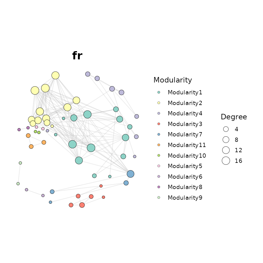
Fruchterman-Reingold (fr)
show_layout("fr1")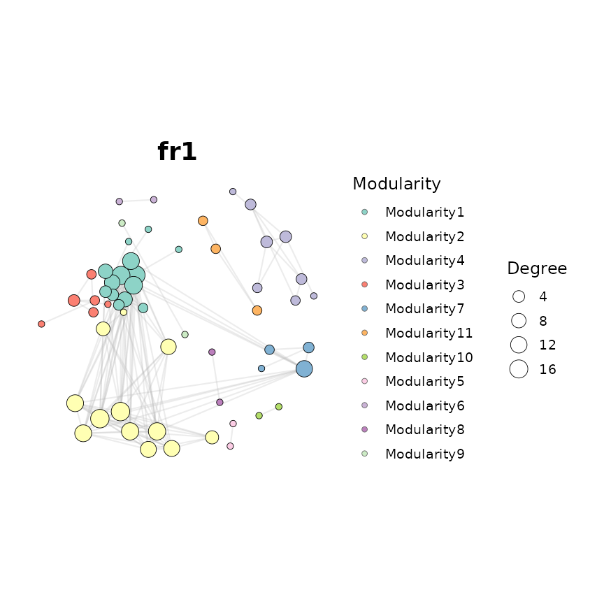
Fruchterman-Reingold variant 1 (fr1)
show_layout("fr2")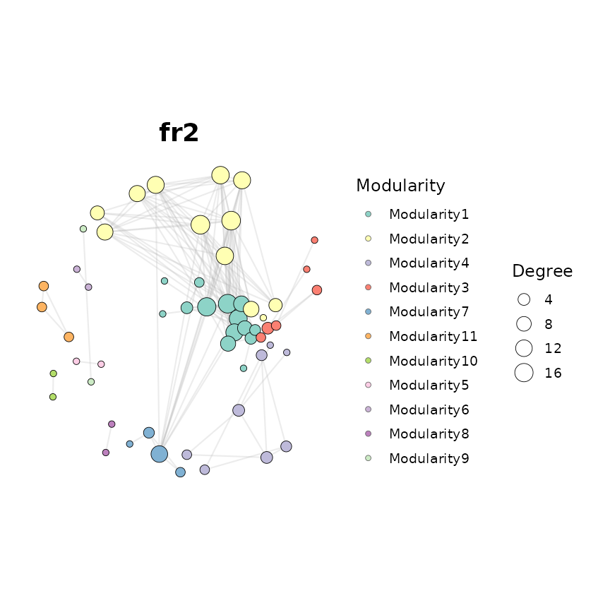
Fruchterman-Reingold variant 2 (fr2)
show_layout("kk")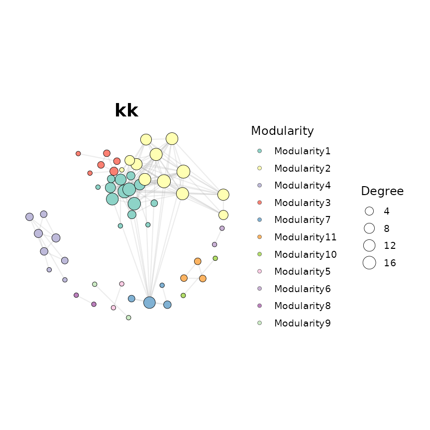
Kamada-Kawai (kk)
show_layout("stress")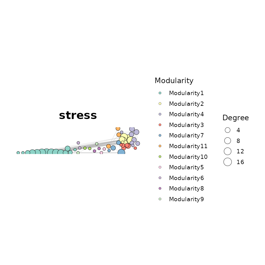
Stress majorisation (stress)
show_layout("nicely")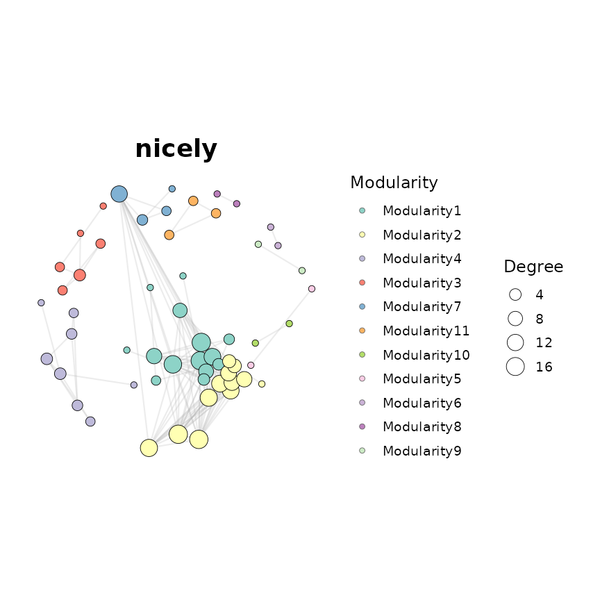
igraph ‘nicely’ auto-selection (nicely)
show_layout("nicely1")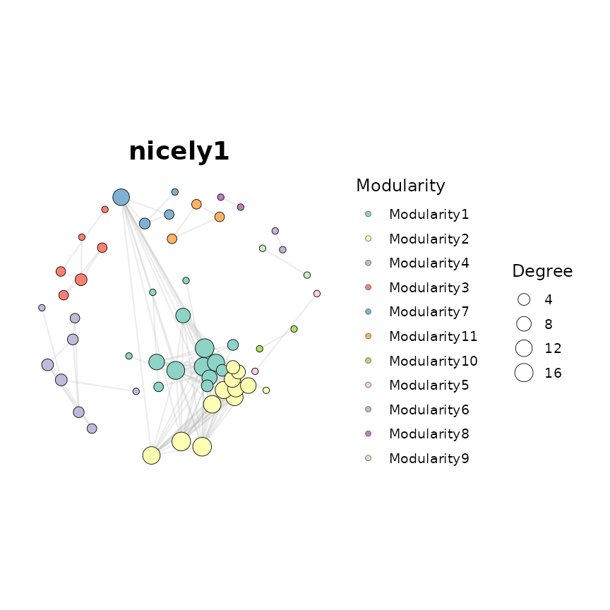
nicely variant (nicely1)
show_layout("lgl")
#> Warning in alg_fun(graph): LGL layout does not support disconnected graphs yet.
#> Source: layout/large_graph.c:179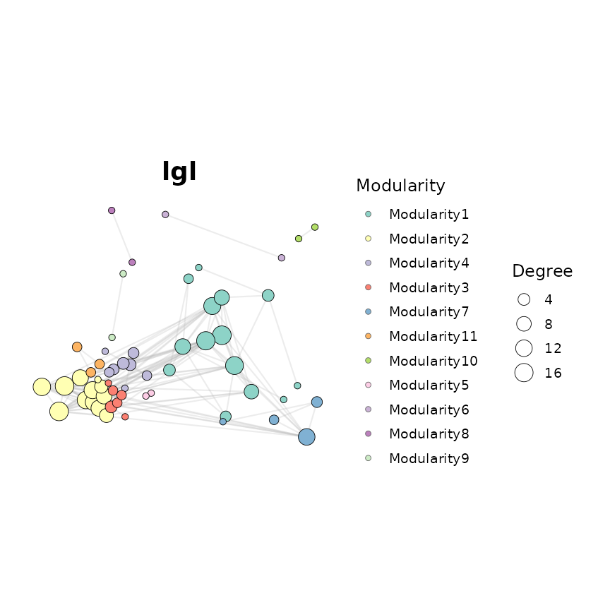
Large Graph Layout (lgl)
show_layout("gephi")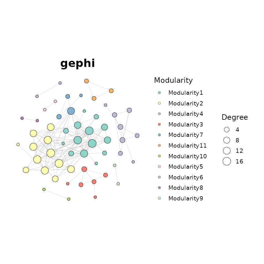
Gephi-style ForceAtlas2 (gephi)
2. Geometric layouts
Simple, deterministic shapes useful when structure clarity matters more than spatial clustering.
show_layout("circle")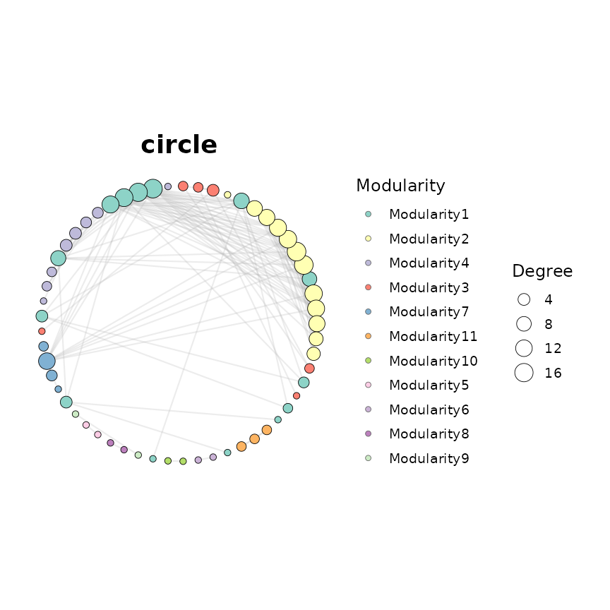
Circle (circle)
show_layout("circle_outline")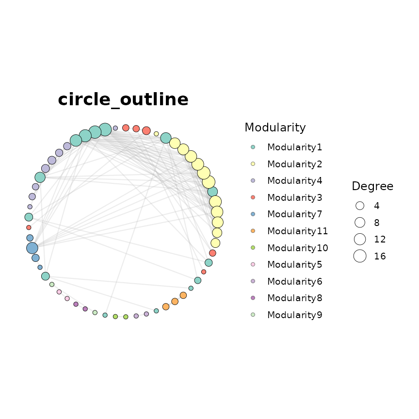
Circle outline (circle_outline)
show_layout("grid")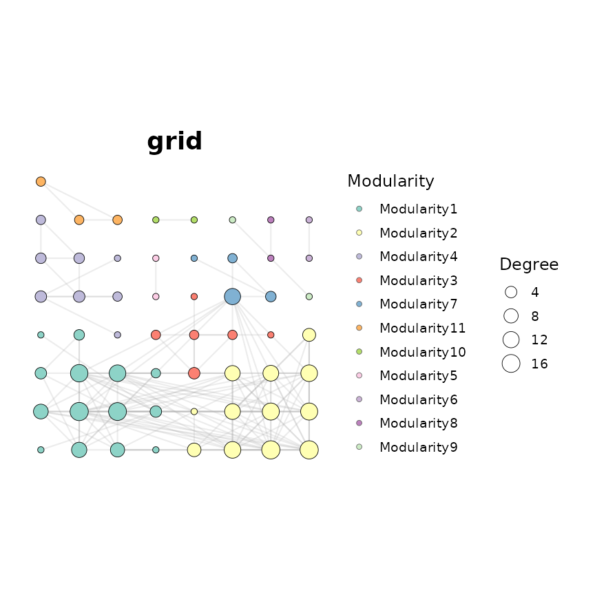
Grid (grid)
show_layout("star")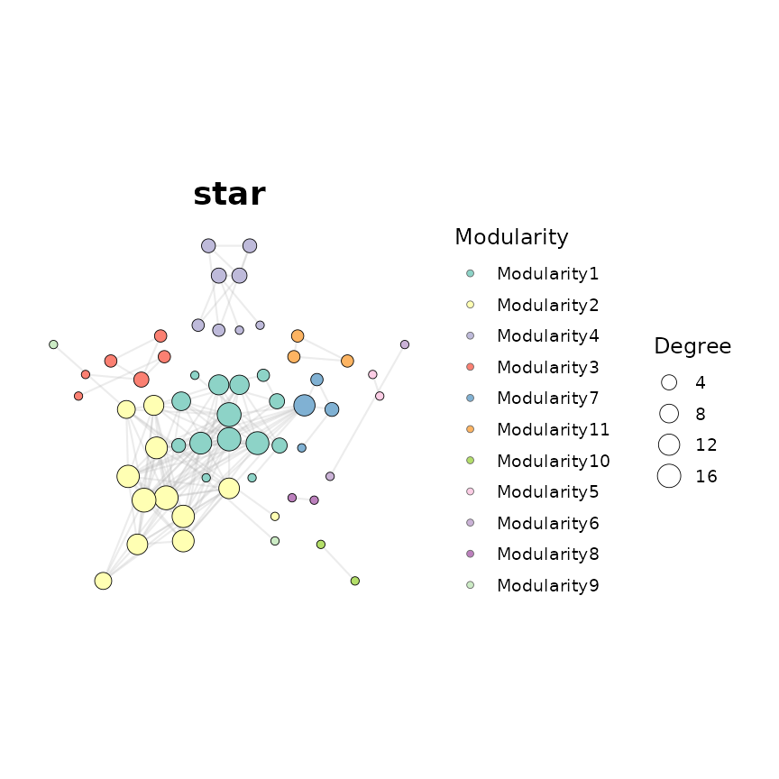
Star (star)
show_layout("star_concentric")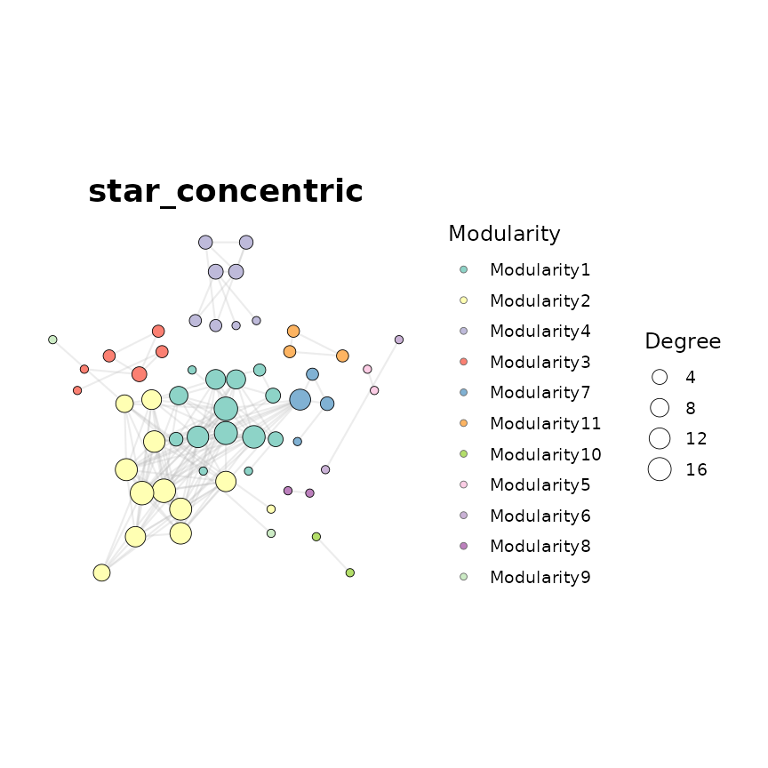
Star concentric (star_concentric)
show_layout("diamond")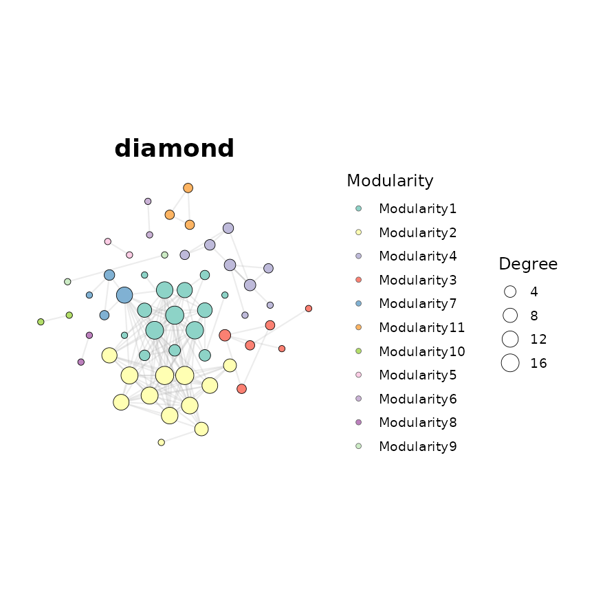
Diamond (diamond)
show_layout("square")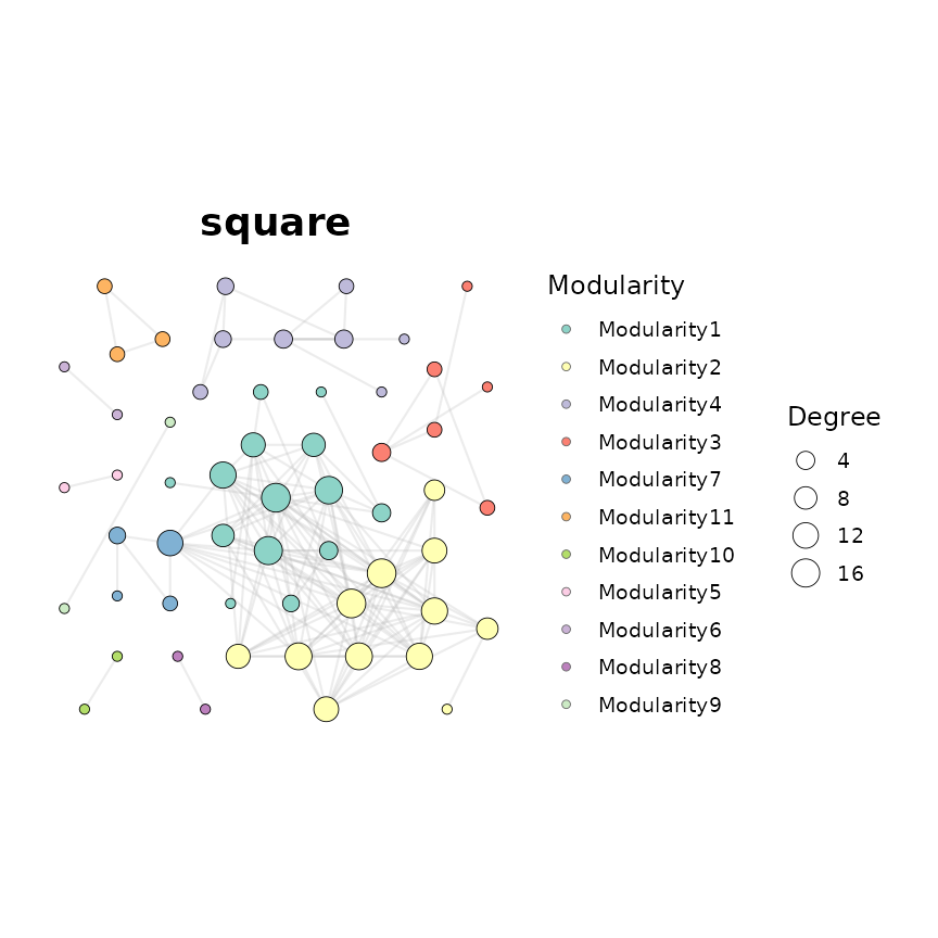
Square (square)
show_layout("square2")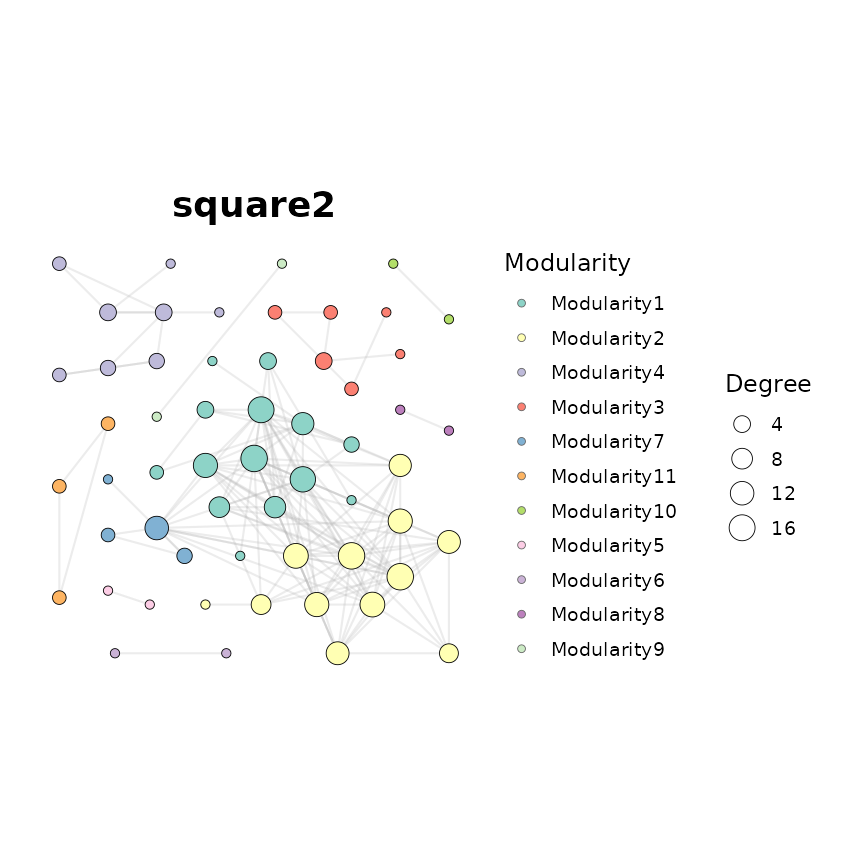
Square variant (square2)
show_layout("rectangle")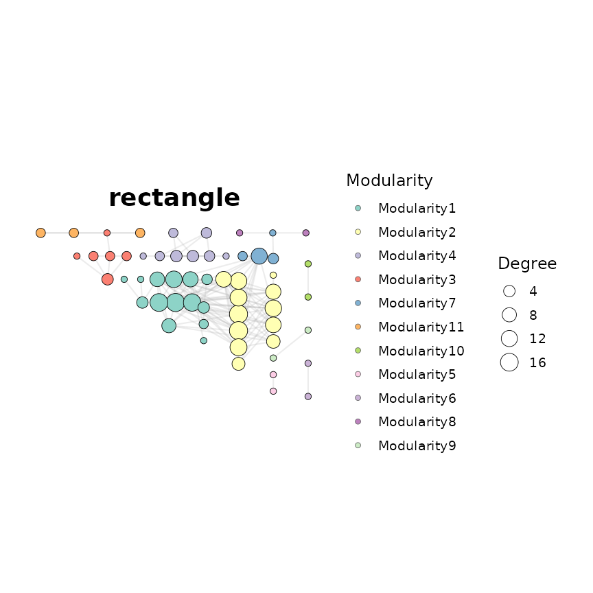
Rectangle (rectangle)
show_layout("rectangle_outline")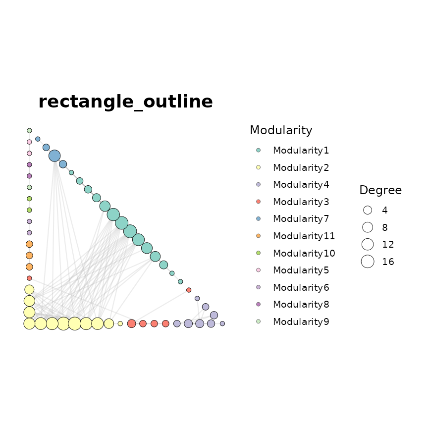
Rectangle outline (rectangle_outline)
show_layout("petal")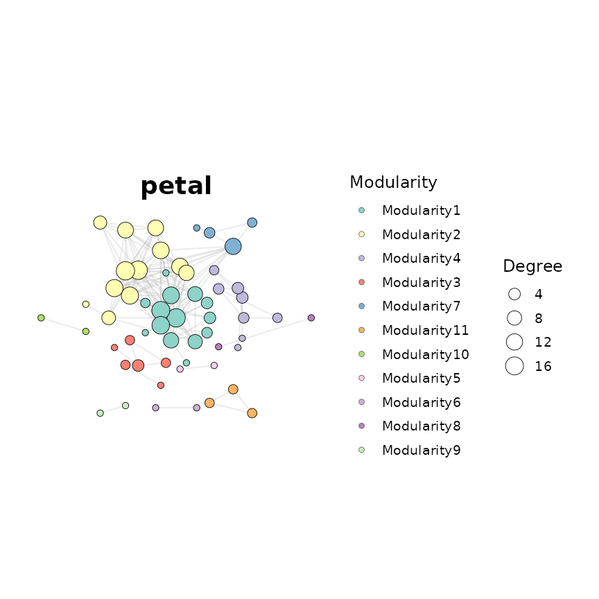
Petal (petal)
show_layout("petal2")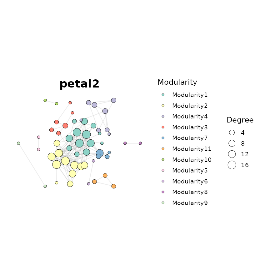
Petal variant (petal2)
show_layout("heart_centered")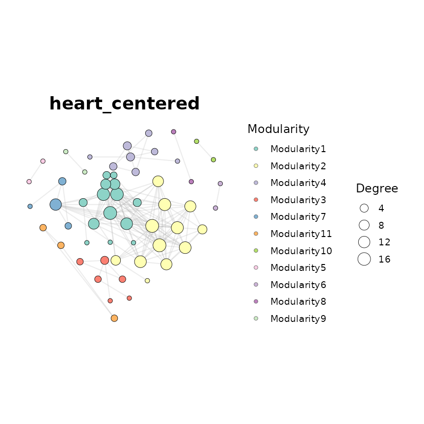
Heart (heart_centered)
show_layout("randomly")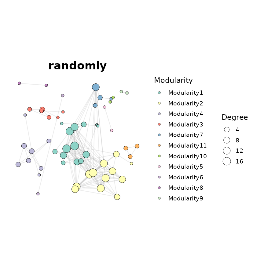
Random (randomly)
4. Circular module layouts
These layouts arrange each module into a distinct geometric shape on a circle, making module boundaries visually explicit. Each comes in a standard version (module sizes proportional to node count) and an equal version (all modules the same size).
Circular module layouts require
layout_module = "adjacent" for best results. They work best
with networks that have well-defined, moderately-sized modules.
# Standard (proportional) variants
show_layout("circular_modules_gephi_layout", layout_module = "adjacent")
show_layout("circular_modules_petal_layout", layout_module = "adjacent")
show_layout("circular_modules_petal2_layout", layout_module = "adjacent")
show_layout("circular_modules_diamond_layout", layout_module = "adjacent")
show_layout("circular_modules_star_layout", layout_module = "adjacent")
show_layout("circular_modules_star_concentric_layout", layout_module = "adjacent")
show_layout("circular_modules_square_layout", layout_module = "adjacent")
show_layout("circular_modules_square2_layout", layout_module = "adjacent")
show_layout("circular_modules_grid_layout", layout_module = "adjacent")
show_layout("circular_modules_heart_centered_layout", layout_module = "adjacent")

# Equal-sized module variants
show_layout("circular_modules_equal_gephi_layout", layout_module = "adjacent")
show_layout("circular_modules_equal_petal_layout", layout_module = "adjacent")
show_layout("circular_modules_equal_petal2_layout", layout_module = "adjacent")
show_layout("circular_modules_equal_diamond_layout", layout_module = "adjacent")
show_layout("circular_modules_equal_star_layout", layout_module = "adjacent")
show_layout("circular_modules_equal_star_concentric_layout", layout_module = "adjacent")
show_layout("circular_modules_equal_square_layout", layout_module = "adjacent")
show_layout("circular_modules_equal_square2_layout", layout_module = "adjacent")
show_layout("circular_modules_equal_grid_layout", layout_module = "adjacent")
show_layout("circular_modules_equal_heart_centered_layout", layout_module = "adjacent")
5. Multipartite layouts
Multipartite layouts separate nodes into two or more spatially distinct groups. Use them when nodes have a categorical block attribute (e.g. bacteria vs. fungi, or different experimental groups).
The layout_module parameter controls how modules are
arranged:
-
"random"– modules distributed freely -
"adjacent"– modules positioned close together -
"order"– modules follow the block order (required for multipartite)
These layouts require that the number of modules matches the expected block count (e.g. bipartite needs exactly 2, tripartite needs 3).
# Bipartite (2-block)
show_layout("bipartite_layout", layout_module = "order")
show_layout("bipartite_gephi_layout", layout_module = "order")

# Tripartite (3-block)
show_layout("tripartite_layout", layout_module = "order")
show_layout("tripartite_gephi_layout", layout_module = "order")
show_layout("tripartite_equal_gephi_layout", layout_module = "order")

# Quadripartite (4-block)
show_layout("quadripartite_gephi_layout", layout_module = "order")
show_layout("quadripartite_equal_gephi_layout", layout_module = "order")
show_layout("cross_quadripartite_gephi_layout", layout_module = "order")
show_layout("cross_quadripartite_equal_gephi_layout", layout_module = "order")

# Pentapartite (5-block)
show_layout("pentapartite_gephi_layout", layout_module = "order")
show_layout("pentapartite_equal_gephi_layout", layout_module = "order")
6. Consensus module layouts
Consensus layouts align modules from different networks into a shared coordinate system. Useful for comparing network structures across conditions.
show_layout("consensus_module_gephi")
show_layout("consensus_module_equal_gephi")
7. The layout_module parameter
All layouts accept layout_module to control how modules
are spatially arranged. Here is the same layout with the three
options:
show_layout("gephi", layout_module = "random")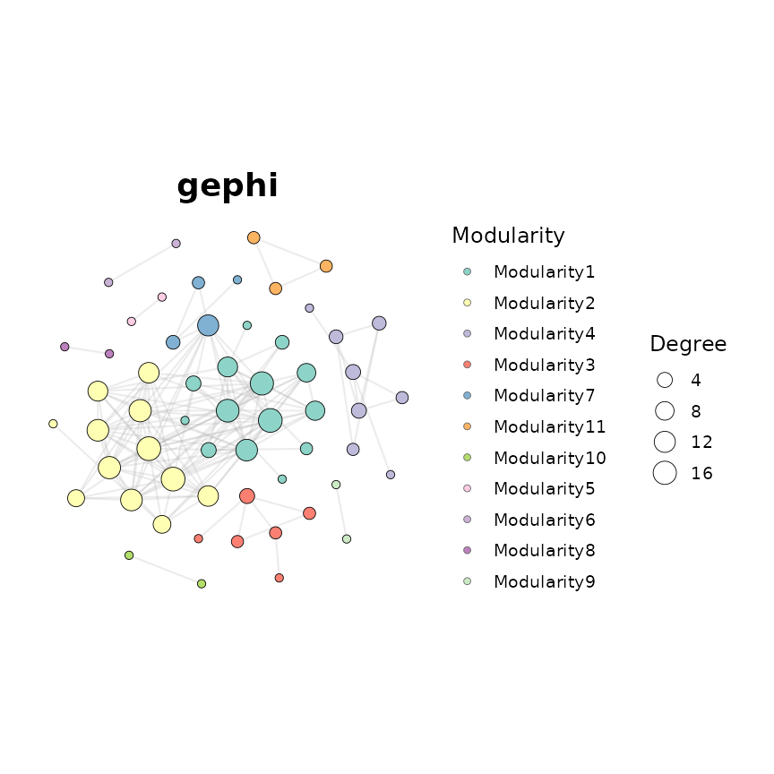
layout_module = ‘random’
show_layout("gephi", layout_module = "adjacent")
#> Warning in ggNetView(g, layout = layout_name, seed = 1, node_size_range = c(2,
#> : `layout_module = 'adjacent'` failed at k_nn = 12; retrying with k_nn = 32.
#> Warning in ggNetView(g, layout = layout_name, seed = 1, node_size_range = c(2,
#> : `layout_module = 'adjacent'` failed at k_nn = 32; retrying with k_nn = 52.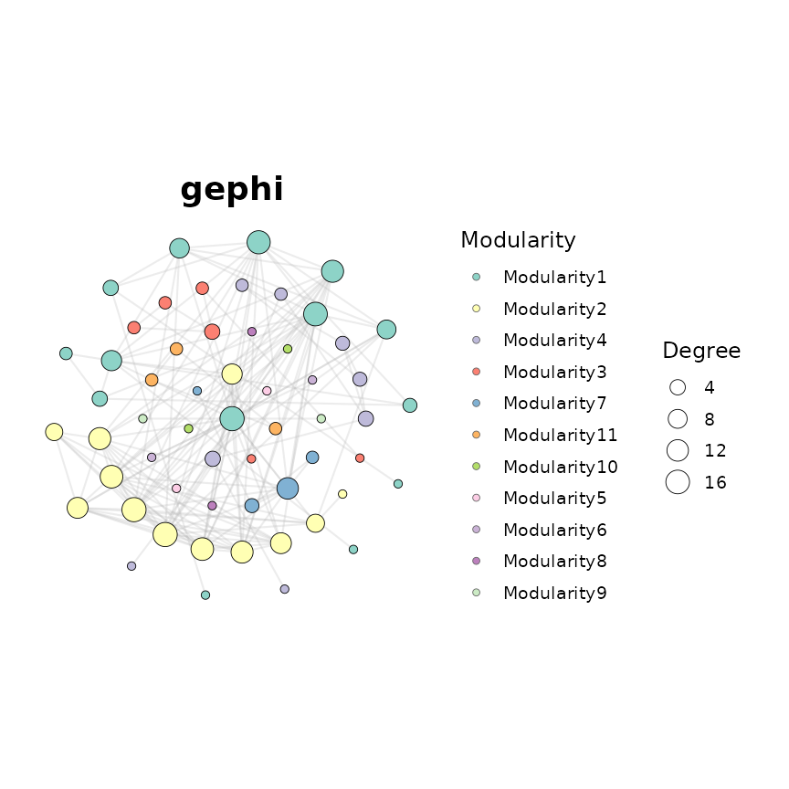
layout_module = ‘adjacent’
Quick reference table
| Family | Layout string | Key feature |
|---|---|---|
| Force-directed |
fr, fr1, fr2
|
Fruchterman-Reingold variants |
kk |
Kamada-Kawai spring model | |
stress |
Stress majorisation | |
nicely, nicely1
|
igraph auto-selection | |
lgl |
Large graph layout | |
gephi |
ForceAtlas2-style | |
| Geometric |
circle, circle_outline
|
Circular |
grid |
Regular grid | |
star, star_concentric
|
Star / concentric rings | |
diamond, diamond_outline
|
Diamond shape | |
square, square2,
square_outline
|
Square shapes | |
rectangle, rectangle_outline
|
Rectangle | |
petal, petal2
|
Petal / flower | |
heart_centered |
Heart shape | |
randomly |
Random placement | |
| Hierarchical | dendrogram |
Circular dendrogram (directed graphs) |
multirings |
Concentric rings | |
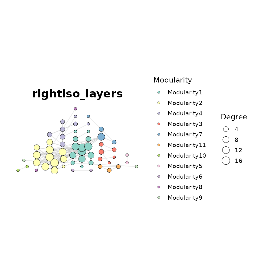
rightiso_layers |
Right-isometric layers | |
| Circular modules | circular_modules_*_layout |
Module per petal/shape |
circular_modules_equal_*_layout |
Equal-sized variant | |
| Multipartite |
bipartite_layout,
bipartite_gephi_layout
|
2-block |
tripartite_* |
3-block | |
quadripartite_*,
cross_quadripartite_*
|
4-block | |
pentapartite_* |
5-block | |
| Consensus | consensus_module_gephi |
Aligned multi-network |
consensus_module_equal_gephi |
Equal-sized variant |
Tips for choosing a layout
-
Start with
"fr"or"gephi"for an overview of community structure. -
Switch to
"circular_modules_*"when you want each module clearly separated. - Use multipartite layouts when nodes have a meaningful block assignment (bacteria/fungi, treatment/control).
-
Use
"dendrogram"for directed / hierarchical graphs. -
Use
layout_module = "adjacent"to pull related modules closer together. -
All layouts are deterministic when
seedis set – figures are reproducible across sessions.
Session information
sessionInfo()
#> R version 4.6.1 (2026-06-24)
#> Platform: x86_64-pc-linux-gnu
#> Running under: Ubuntu 24.04.4 LTS
#>
#> Matrix products: default
#> BLAS:   /usr/lib/x86_64-linux-gnu/openblas-pthread/libblas.so.3
#> LAPACK: /usr/lib/x86_64-linux-gnu/openblas-pthread/libopenblasp-r0.3.26.so;  LAPACK version 3.12.0
#>
#> locale:
#>  [1] LC_CTYPE=C.UTF-8       LC_NUMERIC=C           LC_TIME=C.UTF-8
#>  [4] LC_COLLATE=C.UTF-8     LC_MONETARY=C.UTF-8    LC_MESSAGES=C.UTF-8
#>  [7] LC_PAPER=C.UTF-8       LC_NAME=C              LC_ADDRESS=C
#> [10] LC_TELEPHONE=C         LC_MEASUREMENT=C.UTF-8 LC_IDENTIFICATION=C
#>
#> time zone: UTC
#> tzcode source: system (glibc)
#>
#> attached base packages:
#> [1] stats     graphics  grDevices utils     datasets  methods   base
#>
#> other attached packages:
#> [1] ggNetView_0.2.1
#>
#> loaded via a namespace (and not attached):
#>  [1] tidyselect_1.2.1    psych_2.6.5         viridisLite_0.4.3
#>  [4] dplyr_1.2.1         farver_2.1.2        viridis_0.6.5
#>  [7] S7_0.2.2            ggraph_2.2.2        fastmap_1.2.0
#> [10] tweenr_2.0.3        digest_0.6.39       rpart_4.1.27
#> [13] lifecycle_1.0.5     cluster_2.1.8.2     magrittr_2.0.5
#> [16] compiler_4.6.1      rlang_1.3.0         Hmisc_5.3-0
#> [19] sass_0.4.10         tools_4.6.1         igraph_2.3.3
#> [22] yaml_2.3.12         data.table_1.18.6.1 FNN_1.1.4.1
#> [25] knitr_1.52          labeling_0.4.3      graphlayouts_1.2.5
#> [28] htmlwidgets_1.6.4   mnormt_2.1.2        plyr_1.8.9
#> [31] RColorBrewer_1.1-3  abind_1.4-8         withr_3.0.3
#> [34] foreign_0.8-91      purrr_1.2.2         desc_1.4.3
#> [37] stats4_4.6.1        nnet_7.3-20         grid_4.6.1
#> [40] polyclip_1.10-7     lavaan_0.7-2        colorspace_2.1-3
#> [43] ggplot2_4.0.3       gtools_3.9.5        scales_1.4.0
#> [46] MASS_7.3-65         cli_3.6.6           rmarkdown_2.32
#> [49] ragg_1.5.2          generics_0.1.4      otel_0.2.0
#> [52] rstudioapi_0.19.0   reshape2_1.4.5      pbapply_1.7-5
#> [55] cachem_1.1.0        ggforce_0.5.0       stringr_1.6.0
#> [58] parallel_4.6.1      base64enc_0.1-6     vctrs_0.7.3
#> [61] Matrix_1.7-5        jsonlite_2.0.0      glasso_1.11
#> [64] ggrepel_0.9.8       Formula_1.2-6       htmlTable_2.5.0
#> [67] systemfonts_1.3.2   jpeg_0.1-11         ggnewscale_0.5.2
#> [70] tidyr_1.3.2         jquerylib_0.1.4     qgraph_1.10.1
#> [73] glue_1.8.1          pkgdown_2.2.1       stringi_1.8.9
#> [76] gtable_0.3.6        quadprog_1.5-8      tibble_3.3.1
#> [79] pillar_1.11.1       htmltools_0.5.9     R6_2.6.1
#> [82] textshaping_1.0.5   tidygraph_1.3.1     pbivnorm_0.6.0
#> [85] evaluate_1.0.5      lattice_0.22-9      png_0.1-9
#> [88] backports_1.5.1     memoise_2.0.1       corpcor_1.6.10
#> [91] bslib_0.12.0        fdrtool_1.2.18      Rcpp_1.1.2
#> [94] gridExtra_2.3.1     nlme_3.1-169        checkmate_2.3.4
#> [97] xfun_0.60           fs_2.1.0            pkgconfig_2.0.3