
Node-Importance Analysis: Multiple Centralities and IVI
Source:vignettes/node-importance.Rmd
node-importance.RmdWhy look beyond degree?
Degree is the simplest measure of node importance, and it’s what most
network analyses lead with – including the per-node Degree
and Strength columns that every
build_graph_from_*() constructor in ggNetView
already attaches. But degree only counts a node’s immediate neighbours;
it doesn’t tell you whether those neighbours sit on shortest paths
between distant communities (betweenness), whether the node is “central”
in the global topology (closeness, eigenvector), or whether it functions
as a bridge to other modules (Zi-Pi). For a defensible node-importance
analysis you usually want several complementary perspectives, plus an
integrative score that combines them.
ggNetView exposes node-importance functionality at three
levels:
| Function | What it gives you |
|---|---|
Degree, Strength columns |
Local connectivity (set automatically) |
get_node_centrality() |
Eight per-node centralities (this vignette) |
ggnetview_zipi() |
Module-aware Zi-Pi role classification |
get_node_ivi() |
Salavaty 2020 Integrated Value of Influence |
get_network_topology() |
Network-level summaries of the same metrics |
library(ggNetView)
#>
#>                                                ░██               ░██
#>                                                ░██
#>  ░████████  ░████████ ░████████   ░███████  ░████████ ░██    ░██ ░██ ░███████  ░██    ░██    ░██
#> ░██    ░██ ░██    ░██ ░██    ░██ ░██    ░██    ░██    ░██    ░██ ░██░██    ░██ ░██    ░██    ░██
#> ░██    ░██ ░██    ░██ ░██    ░██ ░█████████    ░██     ░██  ░██  ░██░█████████  ░██  ░████  ░██
#> ░██   ░███ ░██   ░███ ░██    ░██ ░██           ░██      ░██░██   ░██░██          ░██░██ ░██░██
#>  ░█████░██  ░█████░██ ░██    ░██  ░███████      ░████    ░███    ░██ ░███████     ░███   ░███
#>        ░██        ░██
#>  ░███████   ░███████
#>
#>
#> ggNetView: Reproducible and Deterministic Network Analysis and Visualization
#> Version: 0.2.1
#>
#>   Authors:     Yue Liu, Chao Wang
#>   Maintainer:  Yue Liu <yueliu@iae.ac.cn>
#>
#>   Manual:      https://jiawang1209.github.io/ggNetView-manual/
#>   GitHub:      https://github.com/Jiawang1209/ggNetView
#>   Bug Reports: https://github.com/Jiawang1209/ggNetView/issues
#>
#>   Type citation('ggNetView') for how to cite this package.
Build a network
We use the package’s otu_rare_relative example data and
pick the 50 most abundant OTUs to keep the vignette responsive.
data(otu_rare_relative)
data(tax_tab)

mat <- as.matrix(otu_rare_relative)
mat <- mat[order(rowSums(mat), decreasing = TRUE)[seq_len(50)], ]

obj <- build_graph_from_mat(
  mat             = mat,
  method          = "cor",
  cor.method      = "spearman",
  proc            = "BH",
  r.threshold     = 0.5,
  p.threshold     = 0.05,
  module.method   = "Fast_greedy",
  node_annotation = tax_tab[tax_tab$OTUID %in% rownames(mat), ],
  seed            = 1
)
#> The max module in network is 7 we use the 7  modules for next analysis
obj
#> # A tbl_graph: 30 nodes and 53 edges
#> #
#> # An undirected simple graph with 6 components
#> #
#> # Node Data: 30 × 14 (active)
#>    name   modularity modularity2 modularity3 Modularity Degree Strength Kingdom
#>    <chr>  <fct>      <ord>       <chr>       <ord>       <dbl>    <dbl> <chr>
#>  1 ASV_41 2          2           2           2               9     7.36 Archaea
#>  2 ASV_39 2          2           2           2               9     7.24 Bacteria
#>  3 ASV_6  2          2           2           2               8     6.50 Bacteria
#>  4 ASV_10 2          2           2           2               8     6.17 Bacteria
#>  5 ASV_2  2          2           2           2               7     5.78 Archaea
#>  6 ASV_17 2          2           2           2               7     5.72 Bacteria
#>  7 ASV_44 2          2           2           2               7     5.44 Bacteria
#>  8 ASV_24 2          2           2           2               3     2.17 Bacteria
#>  9 ASV_47 2          2           2           2               3     2.29 Bacteria
#> 10 ASV_34 1          1           1           1               4     2.95 Bacteria
#> # ℹ 20 more rows
#> # ℹ 6 more variables: Phylum <chr>, Class <chr>, Order <chr>, Family <chr>,
#> #   Genus <chr>, Species <chr>
#> #
#> # Edge Data: 53 × 5
#>    from    to weight correlation corr_direction
#>   <int> <int>  <dbl>       <dbl> <chr>
#> 1    13    14  0.750       0.750 Positive
#> 2    10    14  0.730       0.730 Positive
#> 3     3     5  0.783       0.783 Positive
#> # ℹ 50 more rows
The result is a tbl_graph whose node table already
carries Degree, Strength, and
Modularity.
Step 1: Compute per-node centralities
obj_aug <- get_node_centrality(obj)

obj_aug %>%
  tidygraph::activate(nodes) %>%
  tidygraph::as_tibble() %>%
  dplyr::select(name, Degree, Strength, Betweenness, Closeness,
                Eigenvector, PageRank, Hub_score, Coreness, Harmonic) %>%
  utils::head(8)
#> # A tibble: 8 × 10
#>   name   Degree Strength Betweenness Closeness Eigenvector PageRank Hub_score
#>   <chr>   <dbl>    <dbl>       <dbl>     <dbl>       <dbl>    <dbl>     <dbl>
#> 1 ASV_41      9     7.36           8    0.0788       1       0.0478     1
#> 2 ASV_39      9     7.24           1    0.0799       0.978   0.0472     0.978
#> 3 ASV_6       8     6.50           2    0.0757       0.944   0.0422     0.944
#> 4 ASV_10      8     6.17           6    0.0779       0.898   0.0404     0.898
#> 5 ASV_2       7     5.78           0    0.0695       0.903   0.0376     0.903
#> 6 ASV_17      7     5.72           0    0.0705       0.899   0.0372     0.899
#> 7 ASV_44      7     5.44           0    0.0728       0.855   0.0356     0.855
#> 8 ASV_24      3     2.17           0    0.0550       0.354   0.0170     0.354
#> # ℹ 2 more variables: Coreness <dbl>, Harmonic <dbl>
get_node_centrality() adds eight new columns
(Betweenness, Closeness, Eigenvector, PageRank, Hub_score,
Authority_score, Coreness, Harmonic) to the existing node schema. Pass
measures = c("Betweenness", "PageRank") (or any subset) to
compute only what you need.
Weighted vs unweighted. Centrality measures interpret edge weights differently. By default
get_node_centrality()uses the unweighted definition; passweighted = TRUEto feed1 / |weight|as the distance vector toigraph(so that strongly correlated pairs count as short paths). For module-detection-friendly inputs the two usually rank the same handful of nodes at the top.
Step 2: Different centralities highlight different nodes
A common observation in network biology is that no single centrality captures all “important” nodes – a node can be a high-degree hub without being on many shortest paths, or vice versa. We can quantify that disagreement:
node_df <- obj_aug %>%
  tidygraph::activate(nodes) %>%
  tidygraph::as_tibble()

top_n <- 10
top_lists <- list(
  Degree      = node_df$name[order(-node_df$Degree)][seq_len(top_n)],
  Betweenness = node_df$name[order(-node_df$Betweenness)][seq_len(top_n)],
  PageRank    = node_df$name[order(-node_df$PageRank)][seq_len(top_n)],
  Eigenvector = node_df$name[order(-node_df$Eigenvector)][seq_len(top_n)]
)

# Pairwise overlap between top-10 lists.
pairs <- utils::combn(names(top_lists), 2, simplify = FALSE)
do.call(rbind, lapply(pairs, function(pair) {
  data.frame(
    a = pair[1L],
    b = pair[2L],
    overlap_top10 = length(intersect(top_lists[[pair[1L]]],
                                     top_lists[[pair[2L]]]))
  )
}))
#>             a           b overlap_top10
#> 1      Degree Betweenness             6
#> 2      Degree    PageRank             6
#> 3      Degree Eigenvector             9
#> 4 Betweenness    PageRank             8
#> 5 Betweenness Eigenvector             5
#> 6    PageRank Eigenvector             5
If two centralities had perfect agreement their pairwise overlap would be 10; if they disagreed completely it would be 0. Real microbiome / gene networks usually fall somewhere in between, and that gap is exactly what a single-metric importance ranking misses.
Step 3: Integrated Value of Influence (IVI)
get_node_ivi() collapses local, semi-local, and global
centralities into one score using the formula of Salavaty et al. (2020).
It’s a thin wrapper over influential::ivi() – the canonical
implementation by the IVI paper’s first author – so the values match the
published algorithm exactly.
The function does one thing: it adds a single new column called
IVI to the input graph’s node table and returns the
augmented tbl_graph. It does not call
ggNetView() or produce any plot – what to do with the IVI
column is entirely up to you.
obj_aug <- get_node_ivi(obj_aug)

# The graph is unchanged except for one new column on the node table:
obj_aug %>%
  tidygraph::activate(nodes) %>%
  tidygraph::as_tibble() %>%
  dplyr::select(name, Modularity, Degree, Betweenness, PageRank, IVI) %>%
  utils::head(5)
#> # A tibble: 5 × 6
#>   name   Modularity Degree Betweenness PageRank   IVI
#>   <chr>  <ord>       <dbl>       <dbl>    <dbl> <dbl>
#> 1 ASV_41 2               9           8   0.0478 34.8
#> 2 ASV_39 2               9           1   0.0472  7.11
#> 3 ASV_6  2               8           2   0.0422 11.3
#> 4 ASV_10 2               8           6   0.0404 27.4
#> 5 ASV_2  2               7           0   0.0376  3.27
The most common deliverable is just a ranked table
For most reports and papers, the deliverable is a small table of the most-influential nodes. One pipe:
obj_aug %>%
  tidygraph::activate(nodes) %>%
  tidygraph::as_tibble() %>%
  dplyr::arrange(dplyr::desc(IVI)) %>%
  dplyr::select(name, Modularity, Degree, IVI) %>%
  utils::head(10)
#> # A tibble: 10 × 4
#>    name   Modularity Degree    IVI
#>    <chr>  <ord>       <dbl>  <dbl>
#>  1 ASV_50 3               9 100
#>  2 ASV_41 2               9  34.8
#>  3 ASV_10 2               8  27.4
#>  4 ASV_24 2               3  25.9
#>  5 ASV_47 2               3  25.9
#>  6 ASV_36 3               3  11.5
#>  7 ASV_6  2               8  11.3
#>  8 ASV_39 2               9   7.11
#>  9 ASV_38 3               2   5.71
#> 10 ASV_2  2               7   3.27
That’s the whole node-importance answer in five lines. No plot required.
Picking a defensible threshold for “significantly influential”
Default get_node_ivi() uses
influential::ivi(scale = "range"), which normalises IVI to
[1, 100] – great for inspecting the full spread of node
influences within one network. Two other scaling modes support different
downstream questions:
-
scale = "z-scale"standardises IVI as a z-score. Use this when comparing influence across multiple networks (e.g. gut vs soil microbiome), or when you want a numeric threshold backed by a one-sided 0.05 cutoff – the IVI paper suggestsz > 1.645. -
scale = "none"returns the raw IVI scores untouched.
obj_z <- get_node_ivi(obj_aug, scale = "z-scale")
obj_z %>%
  tidygraph::activate(nodes) %>%
  tidygraph::as_tibble() %>%
  dplyr::filter(IVI > 1.645) %>%
  dplyr::arrange(dplyr::desc(IVI)) %>%
  dplyr::select(name, Modularity, Degree, IVI)
#> # A tibble: 1 × 4
#>   name   Modularity Degree   IVI
#>   <chr>  <ord>       <dbl> <dbl>
#> 1 ASV_50 3               9  4.64
Larger IVI always means more influential, so ranking by
dplyr::arrange(dplyr::desc(IVI)) works identically across
all three scaling choices.
Step 4 (optional): Map IVI onto a network plot
If you also want a network plot with IVI as a visual aesthetic, you
can pass the IVI-augmented graph to
ggNetView(). Two notes:
-
ggNetView()is a discrete-fill plotter – itsnode_fillargument maps toggplot2::scale_fill_manual(), so it expects a factor / character column, not raw numeric. - Easiest fix: bin
IVIinto a small ordered factor first (quartiles are usually informative), then pass that bin column asnode_fill.
obj_plot <- obj_aug %>%
  tidygraph::activate(nodes) %>%
  tidygraph::mutate(
    IVI_bin = cut(
      IVI,
      breaks = stats::quantile(IVI, probs = seq(0, 1, 0.25), na.rm = TRUE),
      labels = c("Q1 (low)", "Q2", "Q3", "Q4 (high)"),
      include.lowest = TRUE,
      ordered_result = TRUE
    )
  )

ggNetView(
  obj_plot,
  layout    = "fr",
  seed      = 1,
  node_size_range = c(2, 8),
  node_fill   = "IVI_bin",
  module_label     = FALSE
)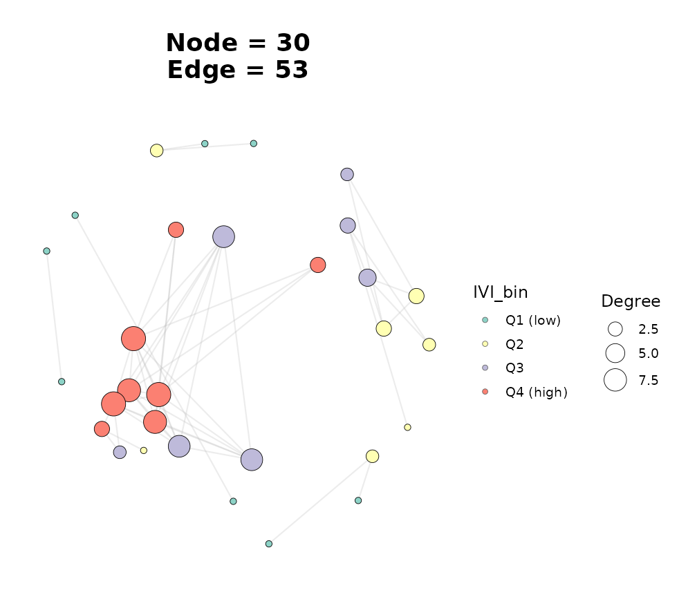
Network coloured by IVI quartile; warmer = more influential.
The same recipe works for any other continuous centrality column
(Betweenness, PageRank,
Eigenvector, …): wrap it in cut() to produce
an ordered factor, then pass that factor as node_fill.
Step 5: Combine with Zi-Pi role classification
For a complete node-importance picture in a modular network, layer IVI on top of Guimera & Amaral’s Zi-Pi roles:
nodes_bulk <- get_graph_nodes(obj_aug)
adj_mat    <- get_graph_adjacency(obj_aug)

zp <- ggnetview_zipi(
  nodes_bulk      = nodes_bulk,
  z_bulk_mat      = adj_mat,
  modularity_col  = "Modularity",
  degree_col      = "Degree"
)

zp$plot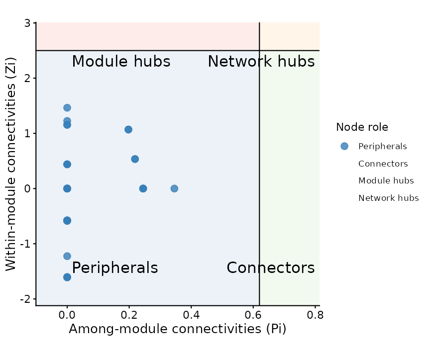
Zi-Pi quadrant plot; node roles classified by within- vs across-module connectivity.
The four quadrants of the Zi-Pi plot – Module hubs,
Connectors, Network hubs, and
Peripherals – partition the network by topological
role, while IVI ranks every node on a single influence
axis. The two views answer different questions and tend to
complement each other: a top-IVI node that lands in the
Network hubs quadrant is a doubly defensible candidate for
biological follow-up.
Choosing a measure
-
Single best general-purpose score:
IVI. Built specifically to reduce the bias of any one centrality. -
For pathfinding / signal-flow questions:
Betweenness(number of shortest paths) orPageRank(weighted random-walk score). -
For “central in the eigen-structure” questions:
Eigenvectorcentrality. -
For module-aware roles: pair Zi-Pi
(
ggnetview_zipi()) with IVI. -
For network-level comparisons (e.g. comparing two
cohorts):
get_network_topology()gives the same families of metrics as scalar means / sums, useful as cohort-vs-cohort summaries.
References
- Salavaty, A., Ramialison, M., & Currie, P. D. (2020). Integrated
Value of Influence: An Integrative Method for the Identification of the
Most Influential Nodes within Networks. Patterns, 1(5),
- Guimera, R., & Amaral, L. A. N. (2005). Functional cartography of complex metabolic networks. Nature, 433(7028), 895-900.