Overview
Weighted Gene Co-expression Network Analysis (WGCNA) is the standard
approach for constructing gene co-expression networks from
high-throughput expression data. ggNetView integrates with
WGCNA at two levels:
-
Quick route – pass
method = "WGCNA"tobuild_graph_from_mat()and let ggNetView handle correlation, thresholding, and module detection in a single call. -
Full pipeline – run the classic WGCNA
soft-thresholding and TOM workflow yourself, then hand the results to
trans_TOM_in_WGCNA()andbuild_graph_from_wgcna()for visualisation.
Both routes produce the same tidygraph object that
ggNetView() can plot directly.
library(ggNetView)
#>
#>                                                ░██               ░██
#>                                                ░██
#>  ░████████  ░████████ ░████████   ░███████  ░████████ ░██    ░██ ░██ ░███████  ░██    ░██    ░██
#> ░██    ░██ ░██    ░██ ░██    ░██ ░██    ░██    ░██    ░██    ░██ ░██░██    ░██ ░██    ░██    ░██
#> ░██    ░██ ░██    ░██ ░██    ░██ ░█████████    ░██     ░██  ░██  ░██░█████████  ░██  ░████  ░██
#> ░██   ░███ ░██   ░███ ░██    ░██ ░██           ░██      ░██░██   ░██░██          ░██░██ ░██░██
#>  ░█████░██  ░█████░██ ░██    ░██  ░███████      ░████    ░███    ░██ ░███████     ░███   ░███
#>        ░██        ░██
#>  ░███████   ░███████
#>
#>
#> ggNetView: Reproducible and Deterministic Network Analysis and Visualization
#> Version: 0.2.1
#>
#>   Authors:     Yue Liu, Chao Wang
#>   Maintainer:  Yue Liu <yueliu@iae.ac.cn>
#>
#>   Manual:      https://jiawang1209.github.io/ggNetView-manual/
#>   GitHub:      https://github.com/Jiawang1209/ggNetView
#>   Bug Reports: https://github.com/Jiawang1209/ggNetView/issues
#>
#>   Type citation('ggNetView') for how to cite this package.
1. Quick route:
build_graph_from_mat(method = "WGCNA")
The simplest way to build a WGCNA-style network is to switch the
method argument. Internally this calls
WGCNA::corAndPvalue() for correlation and p-values, then
applies the same thresholding and module detection as every other
method.
data(otu_rare_relative)
mat <- as.matrix(otu_rare_relative)
mat <- mat[order(rowSums(mat), decreasing = TRUE)[seq_len(80)], ]

graph_wgcna <- build_graph_from_mat(
  mat           = mat,
  method        = "WGCNA",
  cor.method    = "spearman",
  proc          = "BH",
  r.threshold   = 0.6,
  p.threshold   = 0.05,
  module.method = "Fast_greedy",
  seed          = 1
)
#> The max module in network is 11 we use the 11  modules for next analysis

graph_wgcna
#> # A tbl_graph: 57 nodes and 152 edges
#> #
#> # An undirected simple graph with 9 components
#> #
#> # Node Data: 57 × 7 (active)
#>    name   modularity modularity2 modularity3 Modularity Degree Strength
#>    <chr>  <fct>      <ord>       <chr>       <ord>       <dbl>    <dbl>
#>  1 ASV_10 1          1           1           1              17    13.1
#>  2 ASV_2  1          1           1           1              16    12.5
#>  3 ASV_66 1          1           1           1              15    11.6
#>  4 ASV_44 1          1           1           1              13     9.90
#>  5 ASV_77 1          1           1           1              10     7.38
#>  6 ASV_64 1          1           1           1               9     6.53
#>  7 ASV_62 1          1           1           1               8     5.75
#>  8 ASV_33 1          1           1           1               4     3.26
#>  9 ASV_43 1          1           1           1               4     2.77
#> 10 ASV_32 1          1           1           1               3     2.36
#> # ℹ 47 more rows
#> #
#> # Edge Data: 152 × 5
#>    from    to weight correlation corr_direction
#>   <int> <int>  <dbl>       <dbl> <chr>
#> 1    27    31  0.750       0.750 Positive
#> 2    28    31  0.730       0.730 Positive
#> 3     2    17  0.783       0.783 Positive
#> # ℹ 149 more rows
The returned object is identical in structure to one produced with
method = "cor" or "Hmisc", so every downstream
function (ggNetView(), get_network_topology(),
ggnetview_zipi()) works unchanged.
ggNetView(
  graph_wgcna,
  layout    = "fr",
  seed      = 1,
  node_size_range = c(2, 7),
  node_fill   = "Modularity",
  module_label     = FALSE
)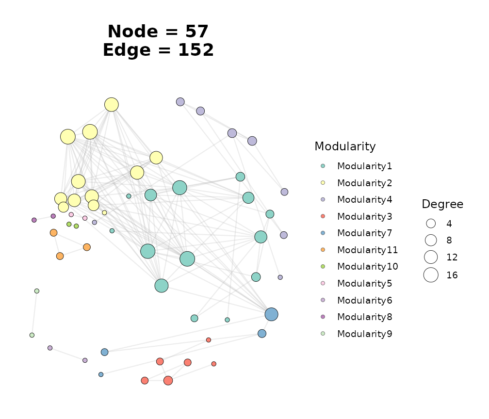
Quick-route WGCNA network coloured by module.
Attaching taxonomy
Pass a node annotation table to colour by taxonomy instead of module:
data(tax_tab)
annot <- tax_tab[tax_tab$OTUID %in% rownames(mat), ]

graph_wgcna_annot <- build_graph_from_mat(
  mat             = mat,
  method          = "WGCNA",
  cor.method      = "spearman",
  proc            = "BH",
  r.threshold     = 0.6,
  p.threshold     = 0.05,
  module.method   = "Fast_greedy",
  node_annotation = annot,
  seed            = 1
)
#> The max module in network is 11 we use the 11  modules for next analysis
ggNetView(
  graph_wgcna_annot,
  layout    = "fr",
  seed      = 1,
  node_size_range = c(2, 7),
  node_fill   = "Phylum",
  module_label     = FALSE
)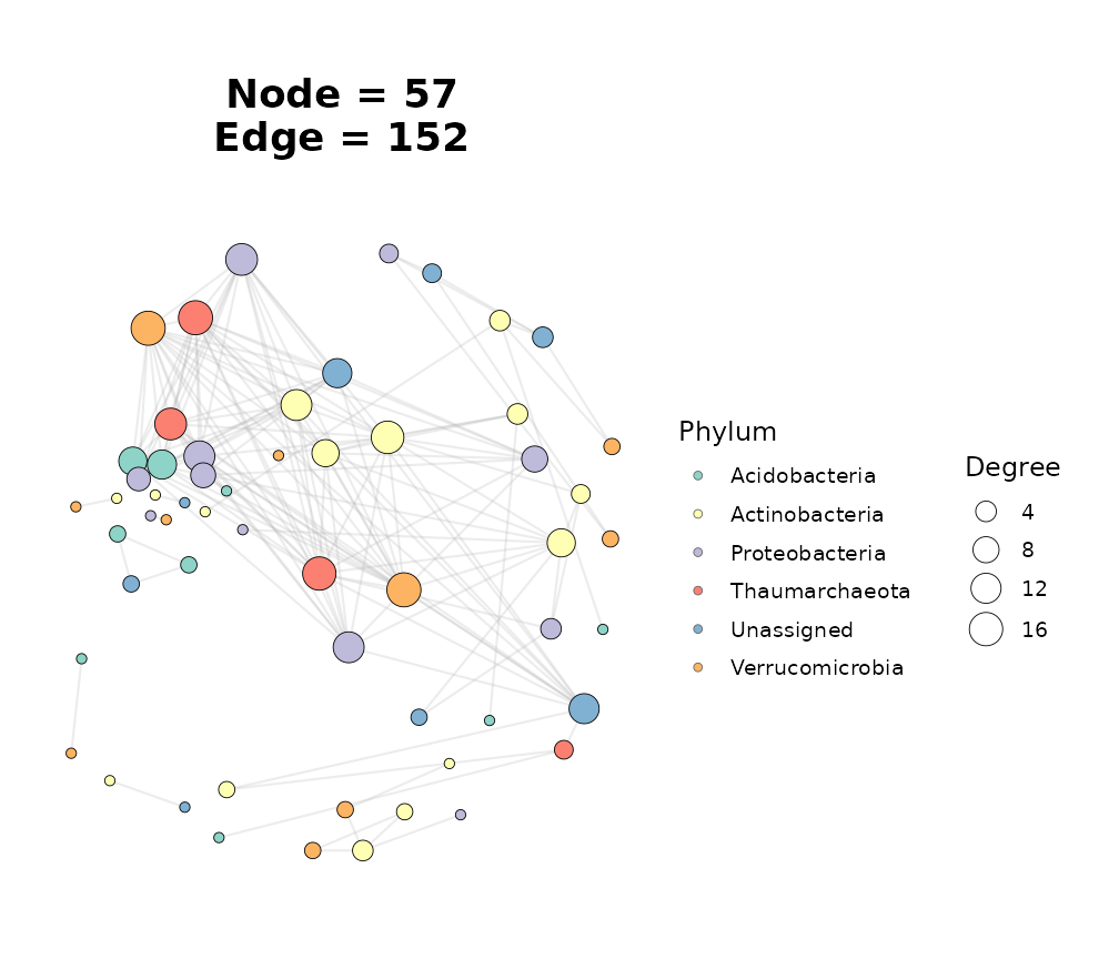
WGCNA network coloured by Phylum.
2. Full WGCNA pipeline
When you need fine-grained control over soft-thresholding power, TOM type, or the dendrogram cut height, run the classic WGCNA steps yourself and feed the results into ggNetView.
Step 2: Pick a soft-thresholding power
# Force WGCNA into single-threaded mode before calling
# `pickSoftThreshold()`. WGCNA spins up an internal foreach/parallel
# cluster by default, which is fragile inside vignette / R CMD check
# environments (and intermittently dies with
# "Error in summary.connection(connection) : invalid connection").
# Single-threaded is slower but deterministic and side-effect-free,
# which is exactly what we want for reproducible documentation. Users
# can re-enable parallelism for production work via
# `WGCNA::allowWGCNAThreads()` or `WGCNA::enableWGCNAThreads()`.
WGCNA::disableWGCNAThreads()

powers <- c(seq(1, 10, by = 1), seq(12, 30, by = 2))
sft <- WGCNA::pickSoftThreshold(
  expr_mat,
  powerVector  = powers,
  networkType  = "signed",
  verbose      = 0
)
#>    Power SFT.R.sq  slope truncated.R.sq mean.k. median.k. max.k.
#> 1      1  0.64600  8.260         0.7460  40.200   40.2000  44.30
#> 2      2  0.17700  1.850         0.2240  22.500   21.8000  28.40
#> 3      3  0.00598 -0.183        -0.0753  13.700   12.7000  20.30
#> 4      4  0.16100 -0.813        -0.0392   8.990    8.0100  15.90
#> 5      5  0.38200 -1.120         0.2140   6.250    5.2600  13.00
#> 6      6  0.46400 -1.250         0.4430   4.570    3.5900  11.10
#> 7      7  0.51400 -1.290         0.5750   3.490    2.5400   9.73
#> 8      8  0.56400 -1.180         0.6800   2.750    1.8200   8.72
#> 9      9  0.51600 -1.110         0.6140   2.230    1.3500   7.91
#> 10    10  0.59900 -1.140         0.6930   1.850    1.0400   7.24
#> 11    12  0.70000 -1.130         0.7580   1.340    0.6550   6.19
#> 12    14  0.02260 -0.940        -0.0480   1.020    0.4450   5.38
#> 13    16  0.75600 -1.060         0.7700   0.808    0.2980   4.73
#> 14    18  0.80400 -1.070         0.7940   0.654    0.2060   4.19
#> 15    20  0.07210 -1.410        -0.0909   0.538    0.1460   3.74
#> 16    22  0.87800 -1.000         0.8720   0.450    0.1070   3.36
#> 17    24  0.95000 -0.961         0.9470   0.381    0.0804   3.03
#> 18    26  0.81200 -0.993         0.8070   0.325    0.0597   2.74
#> 19    28  0.17300 -1.980        -0.0461   0.280    0.0444   2.49
#> 20    30  0.16800 -1.930        -0.0536   0.243    0.0331   2.27

plot(sft$fitIndices[, 1],
     -sign(sft$fitIndices[, 3]) * sft$fitIndices[, 2],
     xlab = "Soft Threshold (power)",
     ylab = "Scale Free Topology Model Fit (signed R^2)",
     main = "Scale independence",
     type = "n")
text(sft$fitIndices[, 1],
     -sign(sft$fitIndices[, 3]) * sft$fitIndices[, 2],
     labels = powers, col = "red")
abline(h = 0.85, col = "red")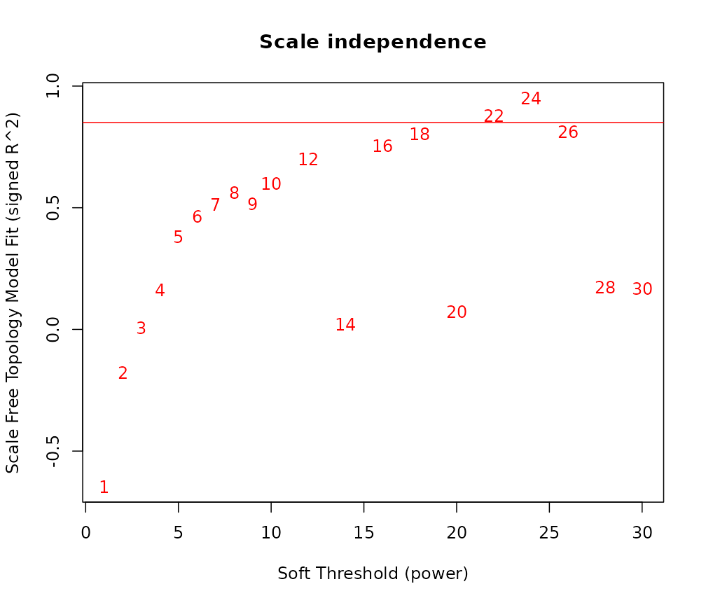
Scale-free topology fit versus soft-thresholding power.
Choose the lowest power where the model fit (\(R^2\)) exceeds 0.85.
Step 3: Build TOM and detect modules
adjacency <- WGCNA::adjacency(
  expr_mat,
  power       = picked_power,
  type        = "signed",
  corFnc      = "cor",
  corOptions  = list(method = "spearman", use = "pairwise.complete.obs")
)

TOM <- WGCNA::TOMsimilarity(adjacency, TOMType = "signed")
#> ..connectivity..
#> ..matrix multiplication (system BLAS)..
#> ..normalization..
#> ..done.
dissTOM <- 1 - TOM

gene_tree <- hclust(as.dist(dissTOM), method = "average")

dynamic_mods <- dynamicTreeCut::cutreeDynamic(
  dendro    = gene_tree,
  distM     = dissTOM,
  deepSplit = 2,
  minClusterSize = 5
)
#>  ..cutHeight not given, setting it to 0.997  ===>  99% of the (truncated) height range in dendro.
#>  ..done.

module_colors <- WGCNA::labels2colors(dynamic_mods)
module_df <- data.frame(
  ID     = colnames(expr_mat),
  Module = module_colors,
  stringsAsFactors = FALSE
)
head(module_df)
#>      ID    Module
#> 1 ASV_1      grey
#> 2 ASV_2 turquoise
#> 3 ASV_3      grey
#> 4 ASV_4      grey
#> 5 ASV_8      grey
#> 6 ASV_6 turquoise
Step 4: Convert TOM to edge list
trans_TOM_in_WGCNA() converts the dense TOM matrix into
a long-format edge list (from, to,
weight). Use the threshold argument to keep
only the strongest edges:
# `trans_TOM_in_WGCNA()` uses `colnames(mat)` as node IDs, so `mat` must
# be in the same orientation as the input to `WGCNA::adjacency()`:
# samples in rows, features (genes/OTUs) in columns. `expr_mat` is
# already in that shape (we transposed once at Step 1), so pass it
# straight in -- transposing again would swap node IDs to sample IDs and
# fail the dimension check inside trans_TOM_in_WGCNA().
edge_df <- trans_TOM_in_WGCNA(
  TOM       = TOM,
  mat       = expr_mat,
  threshold = 0.1
)
head(edge_df)
#>     from     to    weight
#> 1  ASV_2  ASV_6 0.1484648
#> 2  ASV_2 ASV_10 0.1511034
#> 3  ASV_6 ASV_10 0.1168046
#> 4  ASV_2 ASV_17 0.1204909
#> 5  ASV_6 ASV_17 0.4528145
#> 6 ASV_10 ASV_17 0.1158161
dim(edge_df)
#> [1] 59  3
Step 5: Build the ggNetView graph object
graph_full <- build_graph_from_wgcna(
  wgcna_tom       = edge_df,
  module          = module_df,
  node_annotation = annot,
  seed            = 1
)
graph_full
#> # A tbl_graph: 80 nodes and 59 edges
#> #
#> # An undirected simple graph with 61 components
#> #
#> # Node Data: 80 × 15 (active)
#>    name   Module modularity modularity2 modularity3 Modularity Degree Strength
#>    <chr>  <chr>  <fct>      <fct>       <chr>       <fct>       <dbl>    <dbl>
#>  1 ASV_33 blue   blue       blue        blue        blue            3    0.734
#>  2 ASV_77 blue   blue       blue        blue        blue            3    0.706
#>  3 ASV_32 blue   blue       blue        blue        blue            2    0.378
#>  4 ASV_37 blue   blue       blue        blue        blue            2    0.311
#>  5 ASV_43 blue   blue       blue        blue        blue            0    0
#>  6 ASV_46 blue   blue       blue        blue        blue            0    0
#>  7 ASV_66 blue   blue       blue        blue        blue            0    0
#>  8 ASV_3  grey   grey       grey        grey        grey            1    0.169
#>  9 ASV_11 grey   grey       grey        grey        grey            1    0.261
#> 10 ASV_55 grey   grey       grey        grey        grey            1    0.169
#> # ℹ 70 more rows
#> # ℹ 7 more variables: Kingdom <chr>, Phylum <chr>, Class <chr>, Order <chr>,
#> #   Family <chr>, Genus <chr>, Species <chr>
#> #
#> # Edge Data: 59 × 3
#>    from    to weight
#>   <int> <int>  <dbl>
#> 1    60    65  0.148
#> 2    65    68  0.151
#> 3    60    68  0.117
#> # ℹ 56 more rows
Step 6: Visualise
ggNetView(
  graph_full,
  layout    = "fr",
  seed      = 1,
  node_size_range = c(2, 7),
  node_fill   = "Modularity",
  module_label     = FALSE
)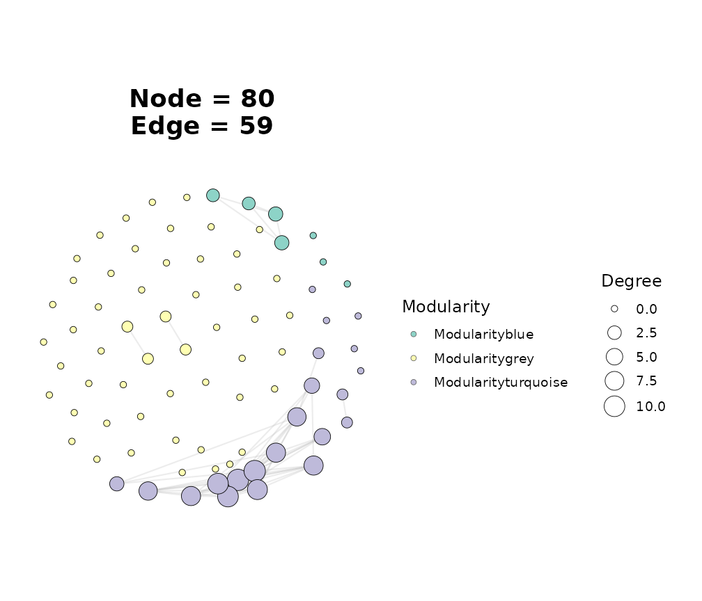
Full WGCNA pipeline – Fruchterman-Reingold layout.
Try different layouts to highlight module structure:
# Note the `_layout` suffix: the petal-style layout functions are named
# `create_layout_circular_modules_petal_layout()` (and the *2 variant),
# whereas other layouts like `fr` / `gephi` / `kk` use the bare name. The
# `layout` argument is concatenated to `create_layout_` to look up the
# function, so it must include the suffix here.
ggNetView(
  graph_full,
  layout    = "circular_modules_petal_layout",
  seed      = 1,
  node_size_range = c(2, 6),
  node_fill   = "Modularity",
  module_label     = FALSE
)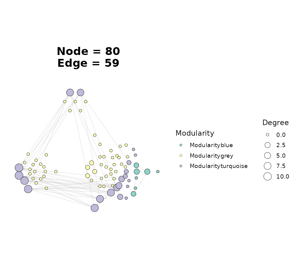
Circular module layout groups nodes by WGCNA module.
3. RMT-guided threshold selection
When you are unsure what r.threshold to use, Random
Matrix Theory (RMT) can pick one automatically.
ggNetView_RMT() scans a range of thresholds and selects the
one whose nearest-neighbour spacing distribution best fits the Poisson
(non-random) model.
rmt_res <- ggNetView_RMT(
  mat     = mat,
  method  = "WGCNA",
  cor.method = "spearman",
  nr_thresholds = 31,
  verbose = FALSE,
  seed    = 1
)
#> Warning in ggNetView_RMT(mat = mat, method = "WGCNA", cor.method = "spearman",
#> : Matrix is relatively small (<100): RMT statistics may be unstable.

message("RMT chosen threshold: ", round(rmt_res$chosen_threshold, 4))
#> RMT chosen threshold: 0.6798
Feed the chosen threshold back into the builder:
graph_rmt <- build_graph_from_mat(
  mat           = mat,
  method        = "WGCNA",
  cor.method    = "spearman",
  proc          = "BH",
  r.threshold   = rmt_res$chosen_threshold,
  p.threshold   = 0.05,
  module.method = "Fast_greedy",
  seed          = 1
)
#> The max module in network is 10 we use the 10  modules for next analysis
ggNetView(
  graph_rmt,
  layout    = "fr",
  seed      = 1,
  node_size_range = c(2, 7),
  node_fill   = "Modularity",
  module_label     = FALSE
)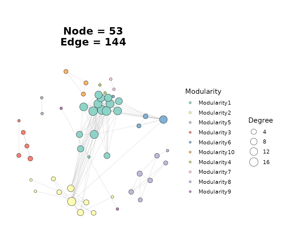
Network built with RMT-selected threshold.
Visualising the RMT scan
The scores element contains per-threshold diagnostics. A
quick plot helps verify the choice:
scores <- rmt_res$scores
plot(scores$threshold, scores$ks_p,
     type = "b", pch = 16,
     xlab = "Correlation threshold",
     ylab = "KS p-value (Exponential fit)",
     main = "RMT threshold scan")
abline(v = rmt_res$chosen_threshold, lty = 2, col = "red")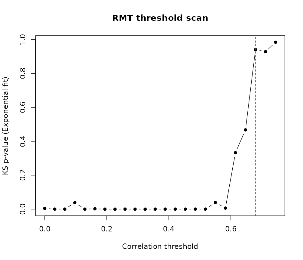
KS p-value (higher = more Poisson-like) across thresholds.
4. Topology and keystone analysis
Once you have a graph object (from either route), the topology and Zi-Pi functions work identically.
Global topology
topo <- get_network_topology(graph_obj = graph_wgcna, bootstrap = 20)
head(topo$topology)
#> # A tibble: 6 × 3
#>   Topology Target_network Random_nerwork
#>   <chr>             <dbl>          <dbl>
#> 1 Node            57             57
#> 2 Edge           152            152
#> 3 Degree           5.33           5.33
#> 4 Distance         1.58           2.56
#> 5 Diameter         3.81           5.1
#> 6 Density          0.0952         0.0952
Zi-Pi classification
nodes_tbl <- get_graph_nodes(graph_wgcna)
adj_mat   <- get_graph_adjacency(graph_wgcna)

zipi <- ggnetview_zipi(
  nodes_bulk     = nodes_tbl,
  z_bulk_mat     = adj_mat,
  modularity_col = "Modularity",
  degree_col     = "Degree"
)
zipi$plot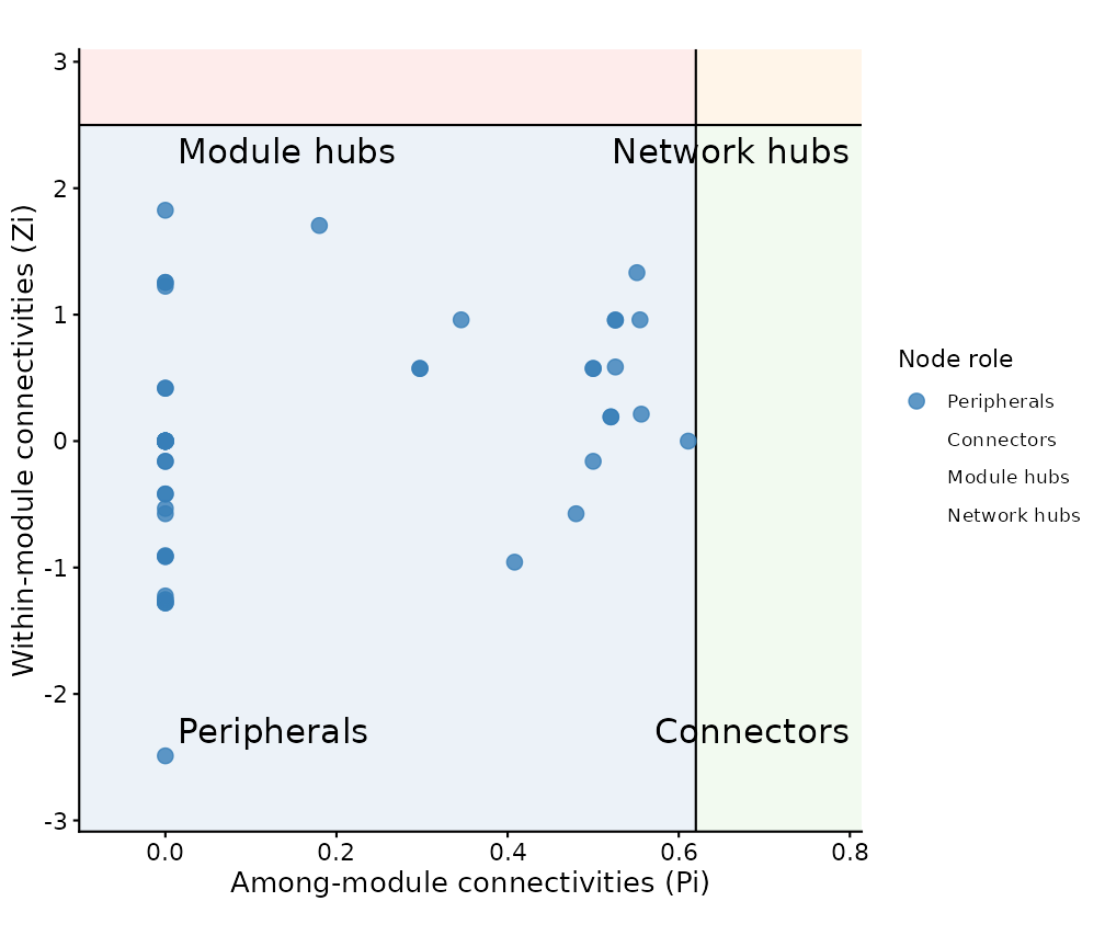
Zi-Pi scatter plot identifying keystone taxa.
Nodes in the upper-right quadrant (high Zi and high Pi) are network hubs – candidates for keystone species or genes that bridge multiple functional modules.
5. Quick-route vs full-pipeline: when to use which
| Feature | Quick route | Full pipeline |
|---|---|---|
| Lines of code | ~10 | ~40 |
| Soft-thresholding power | Not applicable (hard threshold) | User-selected |
| TOM-based edges | No (correlation-based) | Yes |
| Module detection | igraph algorithms | WGCNA dynamicTreeCut
|
| Best for | Exploratory analysis, microbiome data | Gene expression, publication-grade networks |
The quick route treats WGCNA purely as a fast correlation engine and applies the same hard-threshold + igraph-module pipeline as all other methods. The full pipeline preserves the topological overlap information and WGCNA’s own hierarchical module detection, which is the standard for gene co-expression studies.
Session information
sessionInfo()
#> R version 4.6.1 (2026-06-24)
#> Platform: x86_64-pc-linux-gnu
#> Running under: Ubuntu 24.04.4 LTS
#>
#> Matrix products: default
#> BLAS:   /usr/lib/x86_64-linux-gnu/openblas-pthread/libblas.so.3
#> LAPACK: /usr/lib/x86_64-linux-gnu/openblas-pthread/libopenblasp-r0.3.26.so;  LAPACK version 3.12.0
#>
#> locale:
#>  [1] LC_CTYPE=C.UTF-8       LC_NUMERIC=C           LC_TIME=C.UTF-8
#>  [4] LC_COLLATE=C.UTF-8     LC_MONETARY=C.UTF-8    LC_MESSAGES=C.UTF-8
#>  [7] LC_PAPER=C.UTF-8       LC_NAME=C              LC_ADDRESS=C
#> [10] LC_TELEPHONE=C         LC_MEASUREMENT=C.UTF-8 LC_IDENTIFICATION=C
#>
#> time zone: UTC
#> tzcode source: system (glibc)
#>
#> attached base packages:
#> [1] stats     graphics  grDevices utils     datasets  methods   base
#>
#> other attached packages:
#> [1] future_1.75.0   ggNetView_0.2.1
#>
#> loaded via a namespace (and not attached):
#>  [1] tidyselect_1.2.1      viridisLite_0.4.3     WGCNA_1.74
#>  [4] dplyr_1.2.1           farver_2.1.2          viridis_0.6.5
#>  [7] S7_0.2.2              ggraph_2.2.2          fastmap_1.2.0
#> [10] tweenr_2.0.3          digest_0.6.39         rpart_4.1.27
#> [13] lifecycle_1.0.5       cluster_2.1.8.2       survival_3.8-6
#> [16] magrittr_2.0.5        compiler_4.6.1        rlang_1.3.0
#> [19] Hmisc_5.3-0           sass_0.4.10           tools_4.6.1
#> [22] igraph_2.3.3          utf8_1.2.6            yaml_2.3.12
#> [25] data.table_1.18.6.1   knitr_1.52            labeling_0.4.3
#> [28] graphlayouts_1.2.5    htmlwidgets_1.6.4     RColorBrewer_1.1-3
#> [31] foreign_0.8-91        withr_3.0.3           purrr_1.2.2
#> [34] desc_1.4.3            nnet_7.3-20           dynamicTreeCut_1.63-1
#> [37] grid_4.6.1            polyclip_1.10-7       preprocessCore_1.74.0
#> [40] colorspace_2.1-3      fastcluster_1.3.0     ggplot2_4.0.3
#> [43] globals_0.19.1        scales_1.4.0          iterators_1.0.14
#> [46] MASS_7.3-65           cli_3.6.6             rmarkdown_2.32
#> [49] ragg_1.5.2            generics_0.1.4        otel_0.2.0
#> [52] future.apply_1.20.2   rstudioapi_0.19.0     cachem_1.1.0
#> [55] ggforce_0.5.0         stringr_1.6.0         splines_4.6.1
#> [58] parallel_4.6.1        impute_1.86.0         matrixStats_1.5.0
#> [61] base64enc_0.1-6       vctrs_0.7.3           Matrix_1.7-5
#> [64] jsonlite_2.0.0        ggrepel_0.9.8         Formula_1.2-6
#> [67] htmlTable_2.5.0       listenv_1.0.0         systemfonts_1.3.2
#> [70] foreach_1.5.2         ggnewscale_0.5.2      jquerylib_0.1.4
#> [73] tidyr_1.3.2           parallelly_1.48.0     glue_1.8.1
#> [76] pkgdown_2.2.1         codetools_0.2-20      stringi_1.8.9
#> [79] gtable_0.3.6          tibble_3.3.1          pillar_1.11.1
#> [82] htmltools_0.5.9       R6_2.6.1              textshaping_1.0.5
#> [85] doParallel_1.0.17     tidygraph_1.3.1       evaluate_1.0.5
#> [88] lattice_0.22-9        backports_1.5.1       memoise_2.0.1
#> [91] bslib_0.12.0          Rcpp_1.1.2            gridExtra_2.3.1
#> [94] checkmate_2.3.4       xfun_0.60             fs_2.1.0
#> [97] pkgconfig_2.0.3