
Overview
After building a network with any build_graph_from_*()
function, the natural next step is to quantify its structure.
ggNetView provides a family of topology functions that
compute global metrics, per-sample subgraph metrics, robustness
estimates, and node-role classification:
| Function | Purpose |
|---|---|
get_network_topology() |
Global metrics + bootstrap robustness |
get_network_topology_parallel() |
Same, parallelised across a list of networks |
get_sample_subgraph_topology() |
Per-sample subgraph metrics |
get_sample_subgraph_topology_parallel() |
Same, parallelised |
ggnetview_zipi() |
Zi-Pi node-role classification |
ggnetview_modularity_heatmaps() |
Module composition heatmaps |
library(ggNetView)
#>
#>                                                ░██               ░██
#>                                                ░██
#>  ░████████  ░████████ ░████████   ░███████  ░████████ ░██    ░██ ░██ ░███████  ░██    ░██    ░██
#> ░██    ░██ ░██    ░██ ░██    ░██ ░██    ░██    ░██    ░██    ░██ ░██░██    ░██ ░██    ░██    ░██
#> ░██    ░██ ░██    ░██ ░██    ░██ ░█████████    ░██     ░██  ░██  ░██░█████████  ░██  ░████  ░██
#> ░██   ░███ ░██   ░███ ░██    ░██ ░██           ░██      ░██░██   ░██░██          ░██░██ ░██░██
#>  ░█████░██  ░█████░██ ░██    ░██  ░███████      ░████    ░███    ░██ ░███████     ░███   ░███
#>        ░██        ░██
#>  ░███████   ░███████
#>
#>
#> ggNetView: Reproducible and Deterministic Network Analysis and Visualization
#> Version: 0.2.1
#>
#>   Authors:     Yue Liu, Chao Wang
#>   Maintainer:  Yue Liu <yueliu@iae.ac.cn>
#>
#>   Manual:      https://jiawang1209.github.io/ggNetView-manual/
#>   GitHub:      https://github.com/Jiawang1209/ggNetView
#>   Bug Reports: https://github.com/Jiawang1209/ggNetView/issues
#>
#>   Type citation('ggNetView') for how to cite this package.
1. Build a demo network
data(otu_rare_relative)
data(tax_tab)

mat <- as.matrix(otu_rare_relative)
mat <- mat[order(rowSums(mat), decreasing = TRUE)[seq_len(80)], ]
annot <- tax_tab[tax_tab$OTUID %in% rownames(mat), ]

g <- build_graph_from_mat(
  mat             = mat,
  method          = "cor",
  cor.method      = "spearman",
  proc            = "BH",
  r.threshold     = 0.6,
  p.threshold     = 0.05,
  module.method   = "Fast_greedy",
  node_annotation = annot,
  seed            = 1
)
#> The max module in network is 11 we use the 11  modules for next analysis

g
#> # A tbl_graph: 57 nodes and 152 edges
#> #
#> # An undirected simple graph with 9 components
#> #
#> # Node Data: 57 × 14 (active)
#>    name   modularity modularity2 modularity3 Modularity Degree Strength Kingdom
#>    <chr>  <fct>      <ord>       <chr>       <ord>       <dbl>    <dbl> <chr>
#>  1 ASV_10 1          1           1           1              17    13.1  Bacteria
#>  2 ASV_2  1          1           1           1              16    12.5  Archaea
#>  3 ASV_66 1          1           1           1              15    11.6  Bacteria
#>  4 ASV_44 1          1           1           1              13     9.90 Bacteria
#>  5 ASV_77 1          1           1           1              10     7.38 Bacteria
#>  6 ASV_64 1          1           1           1               9     6.53 Bacteria
#>  7 ASV_62 1          1           1           1               8     5.75 Bacteria
#>  8 ASV_33 1          1           1           1               4     3.26 Bacteria
#>  9 ASV_43 1          1           1           1               4     2.77 Bacteria
#> 10 ASV_32 1          1           1           1               3     2.36 Bacteria
#> # ℹ 47 more rows
#> # ℹ 6 more variables: Phylum <chr>, Class <chr>, Order <chr>, Family <chr>,
#> #   Genus <chr>, Species <chr>
#> #
#> # Edge Data: 152 × 5
#>    from    to weight correlation corr_direction
#>   <int> <int>  <dbl>       <dbl> <chr>
#> 1    27    31  0.750       0.750 Positive
#> 2    28    31  0.730       0.730 Positive
#> 3     2    17  0.783       0.783 Positive
#> # ℹ 149 more rows
2. Global network topology
get_network_topology() returns a list with two key
elements:
-
topology– a one-row data frame of global metrics (nodes, edges, average degree, clustering coefficient, modularity, etc.). -
robustness– bootstrap estimates of how metrics behave under random node removal.
topo <- get_network_topology(graph_obj = g, bootstrap = 30)Topology metrics
t(topo$topology)
#>                [,1]           [,2]           [,3]           [,4]
#> Topology       "Node"         "Edge"         "Degree"       "Distance"
#> Target_network " 57.0000000"  "152.0000000"  "  5.3333333"  "  1.5837358"
#> Random_nerwork "5.700000e+01" "1.520000e+02" "5.333333e+00" "2.556268e+00"
#>                [,5]           [,6]           [,7]
#> Topology       "Diameter"     "Density"      "Transitivity_global"
#> Target_network "  3.8059117"  "  0.0952381"  "  0.6993865"
#> Random_nerwork "5.100000e+00" "9.523810e-02" "9.198871e-02"
#>                [,8]                 [,9]           [,10]
#> Topology       "Transitivity_local" "Betweenness"  "Betweenness_edge"
#> Target_network "  0.6982614"        "  9.8947368"  "  6.9078947"
#> Random_nerwork "8.808481e-02"       "4.327427e+01" "2.665417e+01"
#>                [,11]          [,12]              [,13]          [,14]
#> Topology       "Closeness"    "Eigen_centrality" "Modularity"   "K_core_mean"
#> Target_network "  0.3199701"  "  0.2450005"      "  0.3655235"  "  3.9649123"
#> Random_nerwork "7.096269e-03" "4.477036e-01"     "3.439888e-01" "3.483626e+00"
#>                [,15]          [,16]          [,17]
#> Topology       "K_core_max"   "K_core_min"   "Network_efficiency"
#> Target_network " 10.0000000"  "  1.0000000"  "  0.2397394"
#> Random_nerwork "3.966667e+00" "9.666667e-01" "4.452778e-01"
#>                [,18]                     [,19]
#> Topology       "Network_info.centrality" "Cohension_Positive"
#> Target_network "  0.3569606"             NA
#> Random_nerwork "2.146519e-01"            NA
#>                [,20]                [,21]               [,22]
#> Topology       "Cohension_Negative" "Robustness_weight" "Robustness_unweight"
#> Target_network NA                   NA                  NA
#> Random_nerwork NA                   NA                  NA
#>                [,23]           [,24]
#> Topology       "Vulenrability" "Stability"
#> Target_network "  0.1311951"   NA
#> Random_nerwork "3.151864e-02"  NA
Key metrics to look for:
| Metric | Interpretation |
|---|---|
| Nodes / Edges | Network size |
| Average degree | Mean connections per node |
| Clustering coefficient | Local clustering tendency |
| Modularity | Strength of community structure (> 0.4 is strong) |
| Average path length | How many hops between any two nodes |
| Density | Fraction of possible edges realised |
| Positive / Negative edges | Cooperative vs. competitive interactions |
Robustness
The robustness table shows how topology metrics degrade as nodes are randomly removed. This is useful for assessing network stability.
head(topo$robustness)
#> NULL
3. Comparing multiple networks
When you have networks from different conditions (e.g. treatment vs. control, or different time points), pass them as a named list to compute topology in one call.
mat_a <- mat[, 1:9]
mat_b <- mat[, 10:18]

g_a <- build_graph_from_mat(
  mat = mat_a, method = "cor", cor.method = "spearman",
  proc = "BH", r.threshold = 0.6, p.threshold = 0.05,
  module.method = "Fast_greedy", seed = 1
)
#> The max module in network is 7 we use the 7  modules for next analysis
g_b <- build_graph_from_mat(
  mat = mat_b, method = "cor", cor.method = "spearman",
  proc = "BH", r.threshold = 0.6, p.threshold = 0.05,
  module.method = "Fast_greedy", seed = 1
)
#> The max module in network is 2 we use the 2  modules for next analysis

topo_list <- get_network_topology(
  graph_obj_list = list(GroupA = g_a, GroupB = g_b),
  bootstrap      = 20
)

names(topo_list)
#> [1] "GroupA" "GroupB"
Each element contains the same topology +
robustness structure. Bind the topology rows to
compare:
topo_compare <- do.call(rbind, lapply(names(topo_list), function(nm) {
  cbind(Group = nm, topo_list[[nm]]$topology)
}))
t(topo_compare)
#>                [,1]           [,2]           [,3]           [,4]
#> Group          "GroupA"       "GroupA"       "GroupA"       "GroupA"
#> Topology       "Node"         "Edge"         "Degree"       "Distance"
#> Target_network "3.100000e+01" "5.100000e+01" "3.290323e+00" "2.798892e+00"
#> Random_nerwork "31.00000000"  "51.00000000"  " 3.29032258"  " 2.78264506"
#>                [,5]           [,6]           [,7]
#> Group          "GroupA"       "GroupA"       "GroupA"
#> Topology       "Diameter"     "Density"      "Transitivity_global"
#> Target_network "7.365250e+00" "1.096774e-01" "5.663265e-01"
#> Random_nerwork " 6.10000000"  " 0.10967742"  " 0.09645785"
#>                [,8]                 [,9]           [,10]
#> Group          "GroupA"             "GroupA"       "GroupA"
#> Topology       "Transitivity_local" "Betweenness"  "Betweenness_edge"
#> Target_network "6.601010e-01"       "1.429032e+01" "1.298039e+01"
#> Random_nerwork " 0.09944506"        "25.14354839"  "23.82450980"
#>                [,11]          [,12]              [,13]          [,14]
#> Group          "GroupA"       "GroupA"           "GroupA"       "GroupA"
#> Topology       "Closeness"    "Eigen_centrality" "Modularity"   "K_core_mean"
#> Target_network "2.556011e-01" "2.491714e-01"     "5.191189e-01" "2.225806e+00"
#> Random_nerwork " 0.01274970"  " 0.40615457"      " 0.40235486"  " 2.06290323"
#>                [,15]          [,16]          [,17]
#> Group          "GroupA"       "GroupA"       "GroupA"
#> Topology       "K_core_max"   "K_core_min"   "Network_efficiency"
#> Target_network "4.000000e+00" "1.000000e+00" "2.439817e-01"
#> Random_nerwork " 2.60000000"  " 0.45000000"  " 0.40792140"
#>                [,18]                     [,19]
#> Group          "GroupA"                  "GroupA"
#> Topology       "Network_info.centrality" "Cohension_Positive"
#> Target_network "5.294546e-01"            NA
#> Random_nerwork " 0.41003159"             NA
#>                [,20]                [,21]               [,22]
#> Group          "GroupA"             "GroupA"            "GroupA"
#> Topology       "Cohension_Negative" "Robustness_weight" "Robustness_unweight"
#> Target_network NA                   NA                  NA
#> Random_nerwork NA                   NA                  NA
#>                [,23]           [,24]       [,25]          [,26]
#> Group          "GroupA"        "GroupA"    "GroupB"       "GroupB"
#> Topology       "Vulenrability" "Stability" "Node"         "Edge"
#> Target_network "2.538087e-01"  NA          "4.000000e+00" "2.000000e+00"
#> Random_nerwork " 0.09513315"   NA          " 4.00000000"  " 2.00000000"
#>                [,27]          [,28]          [,29]          [,30]
#> Group          "GroupB"       "GroupB"       "GroupB"       "GroupB"
#> Topology       "Degree"       "Distance"     "Diameter"     "Density"
#> Target_network "1.000000e+00" "9.665437e-01" "9.666667e-01" "3.333333e-01"
#> Random_nerwork " 1.00000000"  " 1.25000000"  " 1.75000000"  " 0.33333333"
#>                [,31]                 [,32]                [,33]
#> Group          "GroupB"              "GroupB"             "GroupB"
#> Topology       "Transitivity_global" "Transitivity_local" "Betweenness"
#> Target_network NA                    NA                   "0.000000e+00"
#> Random_nerwork NA                    NA                   " 0.18750000"
#>                [,34]              [,35]          [,36]
#> Group          "GroupB"           "GroupB"       "GroupB"
#> Topology       "Betweenness_edge" "Closeness"    "Eigen_centrality"
#> Target_network "1.000000e+00"     "1.034614e+00" "5.000000e-01"
#> Random_nerwork " 1.75000000"      " 0.54166667"  " 0.66263154"
#>                [,37]          [,38]          [,39]          [,40]
#> Group          "GroupB"       "GroupB"       "GroupB"       "GroupB"
#> Topology       "Modularity"   "K_core_mean"  "K_core_max"   "K_core_min"
#> Target_network "5.000000e-01" "1.000000e+00" "1.000000e+00" "1.000000e+00"
#> Random_nerwork " 0.12500000"  " 0.81250000"  " 1.00000000"  " 0.25000000"
#>                [,41]                [,42]
#> Group          "GroupB"             "GroupB"
#> Topology       "Network_efficiency" "Network_info.centrality"
#> Target_network "3.448715e-01"       "3.218996e-16"
#> Random_nerwork " 0.39583333"        " 0.30000000"
#>                [,43]                [,44]                [,45]
#> Group          "GroupB"             "GroupB"             "GroupB"
#> Topology       "Cohension_Positive" "Cohension_Negative" "Robustness_weight"
#> Target_network NA                   NA                   NA
#> Random_nerwork NA                   NA                   NA
#>                [,46]                 [,47]           [,48]
#> Group          "GroupB"              "GroupB"        "GroupB"
#> Topology       "Robustness_unweight" "Vulenrability" "Stability"
#> Target_network NA                    "1.272518e-04"  NA
#> Random_nerwork NA                    " 0.75000000"   NA
4. Sample-level subgraph topology
In microbiome studies, each sample contains a different subset of
taxa. get_sample_subgraph_topology() extracts a subgraph
per sample (keeping only taxa present in that sample) and computes
topology for each.
sample_topo <- get_sample_subgraph_topology(
  graph_obj = g,
  mat       = mat,
  bootstrap = 10
)

names(sample_topo)
#> [1] "subgraph_list" "topology"      "Robustness"    "sample_stat"
The result contains:
-
subgraph_list– per-sampletbl_graphobjects -
topology– merged topology table (one row per sample) -
Robustness– merged robustness table -
sample_stat– summary of node/edge counts per sample
head(sample_topo$sample_stat)
#>     Sample Node Edge Status
#> KO1    KO1   57  152     OK
#> KO2    KO2   57  152     OK
#> KO3    KO3   57  152     OK
#> KO4    KO4   57  152     OK
#> KO5    KO5   57  152     OK
#> KO6    KO6   57  152     OK
head(sample_topo$topology)
#> # A tibble: 6 × 4
#>   Sample Topology Target_network Random_nerwork
#>   <chr>  <chr>             <dbl>          <dbl>
#> 1 KO1    Node            57             57
#> 2 KO1    Edge           152            152
#> 3 KO1    Degree           5.33           5.33
#> 4 KO1    Distance         1.58           2.53
#> 5 KO1    Diameter         3.81           4.8
#> 6 KO1    Density          0.0952         0.0952
Parallel version
For large datasets with many samples, use the parallel variant to speed up computation:
sample_topo_par <- get_sample_subgraph_topology_parallel(
  graph_obj = g,
  mat       = mat,
  bootstrap = 10
)
The output structure is identical.
5. Zi-Pi node-role classification
The Zi-Pi framework (Guimera & Amaral, 2005) classifies each node by two metrics:
- Zi (within-module connectivity) – how well connected a node is within its own module.
- Pi (participation coefficient) – how much a node connects to other modules.
Default thresholds (Zi = 2.5, Pi = 0.62) divide nodes into four roles:
                        Pi < 0.62          Pi >= 0.62
             ┌─────────────────────┬─────────────────────┐
  Zi >= 2.5  │   Module hubs       │   Network hubs      │
             ├─────────────────────┼─────────────────────┤
  Zi <  2.5  │   Peripherals       │   Connectors        │
             └─────────────────────┴─────────────────────┘
Computing Zi-Pi
nodes_tbl <- get_graph_nodes(g)
adj_mat   <- get_graph_adjacency(g)

zipi <- ggnetview_zipi(
  nodes_bulk     = nodes_tbl,
  z_bulk_mat     = adj_mat,
  modularity_col = "Modularity",
  degree_col     = "Degree"
)
The result contains a data frame and a ready-made
plot:
head(zipi$data[, c("name", "within_module_connectivities",
                    "among_module_connectivities", "type")])
#>     name within_module_connectivities among_module_connectivities        type
#> 1 ASV_10                    0.5861739                   0.5259516 Peripherals
#> 2  ASV_2                    0.9591936                   0.5546875 Peripherals
#> 3 ASV_66                    1.3322134                   0.5511111 Peripherals
#> 4 ASV_44                    0.2131541                   0.5562130 Peripherals
#> 5 ASV_77                    1.7052331                   0.1800000 Peripherals
#> 6 ASV_64                    0.9591936                   0.3456790 Peripherals
table(zipi$data$type)
#>
#>  Peripherals   Connectors  Module hubs Network hubs
#>           57            0            0            0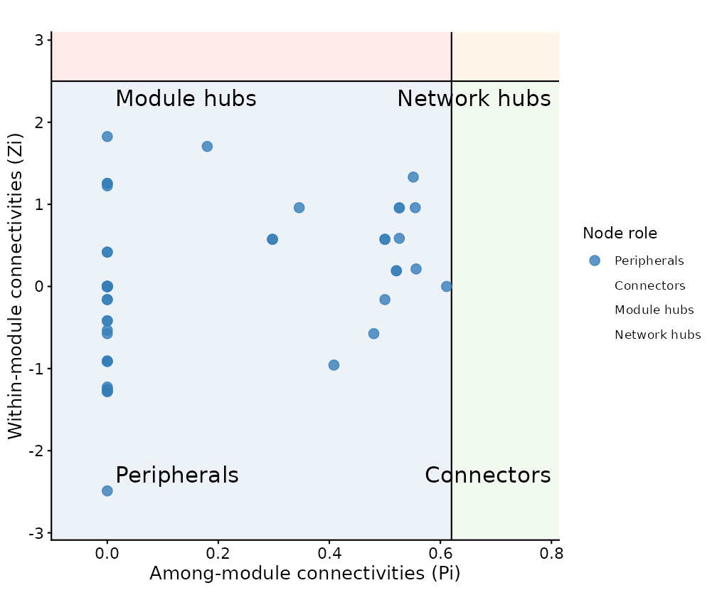
Interpreting node roles
- Peripherals (most nodes) – loosely connected within and across modules. They follow the community structure passively.
- Module hubs – highly connected within their module but not bridging to others. Removal destabilises the module.
- Connectors – bridge nodes linking different modules. Important for network-wide information flow.
- Network hubs – both intra- and inter-module hubs. The most critical nodes; candidates for keystone species or genes.
Custom thresholds
Adjust the classification boundaries when the defaults do not fit your system:
zipi_strict <- ggnetview_zipi(
  nodes_bulk     = nodes_tbl,
  z_bulk_mat     = adj_mat,
  modularity_col = "Modularity",
  degree_col     = "Degree",
  zi_threshold   = 2.0,
  pi_threshold   = 0.5
)

table(zipi_strict$data$type)
#>
#>  Peripherals   Connectors  Module hubs Network hubs
#>           45           12            0            0
6. Module composition summary
You can summarise module composition by counting nodes and examining the dominant taxa per module:
nodes <- get_graph_nodes(g)
module_summary <- as.data.frame(table(
  Module = as.character(nodes$Modularity)
))
colnames(module_summary)[2] <- "Nodes"
module_summary <- module_summary[order(-module_summary$Nodes), ]
module_summary
#>    Module Nodes
#> 1       1    14
#> 4       2    12
#> 6       4     8
#> 5       3     6
#> 9       7     4
#> 3      11     3
#> 2      10     2
#> 7       5     2
#> 8       6     2
#> 10      8     2
#> 11      9     2
For richer module-environment correlation heatmaps, see
ggnetview_modularity_heatmaps() which links module
eigengenes or abundances to environmental variables — it requires an
environmental data frame and env_select specification.
7. Putting it all together: a typical workflow
# 1. Build network
g <- build_graph_from_mat(mat, method = "cor", ...)

# 2. Visualise
ggNetView(g, layout = "fr", node_fill = "Modularity")

# 3. Global topology
topo <- get_network_topology(g, bootstrap = 100)

# 4. Sample-level topology
sample_topo <- get_sample_subgraph_topology(g, mat, bootstrap = 50)

# 5. Keystone detection
zipi <- ggnetview_zipi(
  get_graph_nodes(g), get_graph_adjacency(g),
  "Modularity", "Degree"
)

# 6. Module summary
table(get_graph_nodes(g)$Modularity)
Steps 3-6 work with any graph produced by
build_graph_from_mat(), build_graph_from_df(),
build_graph_from_wgcna(), or any other builder – the
topology functions only need a tbl_graph input.
Session information
sessionInfo()
#> R version 4.6.1 (2026-06-24)
#> Platform: x86_64-pc-linux-gnu
#> Running under: Ubuntu 24.04.4 LTS
#>
#> Matrix products: default
#> BLAS:   /usr/lib/x86_64-linux-gnu/openblas-pthread/libblas.so.3
#> LAPACK: /usr/lib/x86_64-linux-gnu/openblas-pthread/libopenblasp-r0.3.26.so;  LAPACK version 3.12.0
#>
#> locale:
#>  [1] LC_CTYPE=C.UTF-8       LC_NUMERIC=C           LC_TIME=C.UTF-8
#>  [4] LC_COLLATE=C.UTF-8     LC_MONETARY=C.UTF-8    LC_MESSAGES=C.UTF-8
#>  [7] LC_PAPER=C.UTF-8       LC_NAME=C              LC_ADDRESS=C
#> [10] LC_TELEPHONE=C         LC_MEASUREMENT=C.UTF-8 LC_IDENTIFICATION=C
#>
#> time zone: UTC
#> tzcode source: system (glibc)
#>
#> attached base packages:
#> [1] stats     graphics  grDevices utils     datasets  methods   base
#>
#> other attached packages:
#> [1] future_1.75.0   ggNetView_0.2.1
#>
#> loaded via a namespace (and not attached):
#>  [1] tidyselect_1.2.1      psych_2.6.5           WGCNA_1.74
#>  [4] dplyr_1.2.1           farver_2.1.2          S7_0.2.2
#>  [7] fastmap_1.2.0         digest_0.6.39         rpart_4.1.27
#> [10] lifecycle_1.0.5       cluster_2.1.8.2       survival_3.8-6
#> [13] magrittr_2.0.5        compiler_4.6.1        rlang_1.3.0
#> [16] Hmisc_5.3-0           sass_0.4.10           tools_4.6.1
#> [19] igraph_2.3.3          utf8_1.2.6            yaml_2.3.12
#> [22] data.table_1.18.6.1   knitr_1.52            labeling_0.4.3
#> [25] htmlwidgets_1.6.4     mnormt_2.1.2          RColorBrewer_1.1-3
#> [28] withr_3.0.3           foreign_0.8-91        purrr_1.2.2
#> [31] desc_1.4.3            nnet_7.3-20           dynamicTreeCut_1.63-1
#> [34] grid_4.6.1            preprocessCore_1.74.0 colorspace_2.1-3
#> [37] fastcluster_1.3.0     ggplot2_4.0.3         globals_0.19.1
#> [40] scales_1.4.0          iterators_1.0.14      cli_3.6.6
#> [43] rmarkdown_2.32        ragg_1.5.2            generics_0.1.4
#> [46] otel_0.2.0            rstudioapi_0.19.0     future.apply_1.20.2
#> [49] cachem_1.1.0          stringr_1.6.0         splines_4.6.1
#> [52] parallel_4.6.1        impute_1.86.0         matrixStats_1.5.0
#> [55] base64enc_0.1-6       vctrs_0.7.3           Matrix_1.7-5
#> [58] jsonlite_2.0.0        Formula_1.2-6         htmlTable_2.5.0
#> [61] listenv_1.0.0         systemfonts_1.3.2     foreach_1.5.2
#> [64] ggnewscale_0.5.2      tidyr_1.3.2           jquerylib_0.1.4
#> [67] glue_1.8.1            parallelly_1.48.0     pkgdown_2.2.1
#> [70] codetools_0.2-20      stringi_1.8.9         gtable_0.3.6
#> [73] tibble_3.3.1          pillar_1.11.1         htmltools_0.5.9
#> [76] R6_2.6.1              textshaping_1.0.5     doParallel_1.0.17
#> [79] tidygraph_1.3.1       evaluate_1.0.5        lattice_0.22-9
#> [82] backports_1.5.1       bslib_0.12.0          Rcpp_1.1.2
#> [85] gridExtra_2.3.1       nlme_3.1-169          checkmate_2.3.4
#> [88] xfun_0.60             fs_2.1.0              pkgconfig_2.0.3